missingHE is a R package aimed at providing some useful tools to analysts in order to handle missing outcome data under a Full Bayesian framework in economic evaluations. The package relies on the R package R2jags to implement Bayesian methods via the statistical software JAGS. The package allows to obtain inferences using Markov Chain Monte Carlo (MCMC) methods under a range of modelling approaches and missing data assumptions. The package also contains functions specifically defined to assess model fit and possible issues in model convergence as well as to summarise the main results from the economic analysis.
Missing data are iteratively imputed using data augmentation methods according to the type of model, distribution and missingness assumptions specified by the user using different arguments in the functions of the package. The posterior distribution of the main quantities of interest (e.g. some suitable measures of costs and clinical benefits) is then summarised to assess the cost-effectiveness of a new intervention ($t=2$) against a standard intervention ($t=1$).
missingHE produces plots which compares the observed and imputed values for both cost and benefit measures in each treatment intervention considered to detect possible concerns about the plausibility of the imputation methods. In addition, the output of missingHE cab be analysed using different funtions in the R package BCEA which produces a synthesis of the decision process given the current evidence and uncertainty, as well as several indicators that can be used to perform Probabilistic Sensitivity Analysis to parameter and model uncertainty.
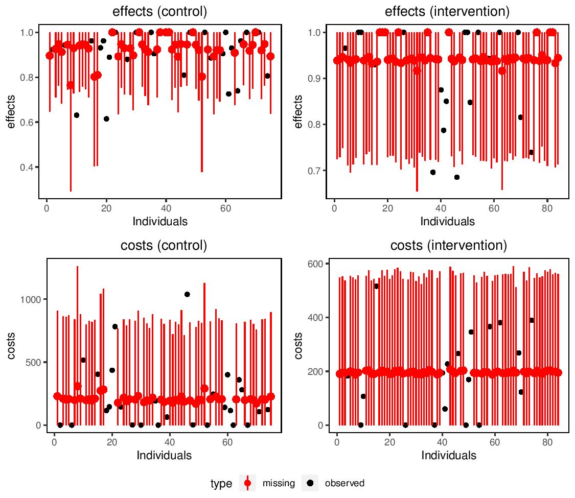
Example of a graphical output from missingHE
Example
library(missingHE)
model.sel <- selection(data = MenSS, model.eff = e ~ u.0, model.cost = c ~ e, model.me = me ~ 1, model.mc = mc ~ 1,
                       type = "MAR", n.chains = 2, n.iter = 10000, n.burnin = 1000, dist_e = "norm", dist_c = "norm")
summary(model.sel)
 Cost-effectiveness analysis summary

 Comparator intervention: intervention 1
 Reference intervention: intervention 2

 Parameter estimates under MAR assumption

 Comparator intervention
               mean     sd      LB      UB
mean.effects  0.874  0.017   0.846   0.901
mean.costs   238.34 52.432 153.541 325.355

 Reference intervention
                  mean    sd      LB      UB
mean.effects.1   0.917 0.022   0.881   0.953
mean.costs.1   186.825 41.26 119.672 254.125

 Incremental results
                   mean     sd       LB     UB
delta.effects     0.043  0.028   -0.003  0.089
delta.costs     -51.514 67.025 -162.862 58.327
ICER          -1198.431
News and updates about missingHE
- From 25/09/2019, the updated version (1.2.1) of
missingHEhas become available on CRAN, which allows to perform posterior predictive checks for each type of model as a further way to assess the fit of the model to the observed data.
The checks can be done by first setting the optional argument ppc = TRUE when fitting the model using one of the main function of the package. For example, when using selection to fit selection models you would have something like this:
model.sel <- selection(data = data, model.eff = e ~ age, model.cost = c ~ age + e, model.me = me ~ age, model.mc = mc ~ age,
dist_e = "norm", dist_c = "gamma", type = "MAR", n.iter = 10000, ppc = TRUE)
Then you can use the function ppc to perform different types of posterior predictive checks that you can choose among a set of pre-specified types using the type argument. For example, if we want to compare histograms of the empirical and predictive distributions of the effectiveness variable in one arm (e.g. control), then we can type
ppc(model.sel, type = "histogram", outcome = "effects_arm1")
and we get something like this
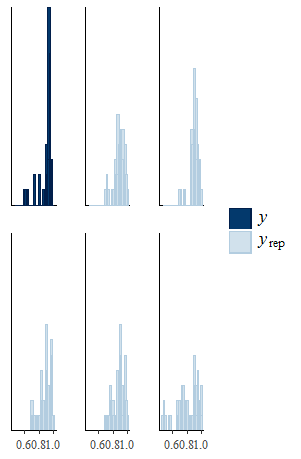
Example of posterior predictive checks in missingHE
- From 07/01/2020, the updated version (1.3.2) of
missingHEhas become available on CRAN, which allows to choose among more distributions for the effectiveness measures, including continuous (Gamma, Weibull, Exponential, Logistic), discrete (Poisson, Negative Binomial) and binary (Bernoulli) health outcomes.
For example, we can choose to specify a selection model assuming a Bernoulli distribution for the effects (if this is a binary outcome) and a LogNormak distribution for the costs
model.sel <- selection(data = data, model.eff = e ~ age, model.cost = c ~ age + e, model.me = me ~ 1, model.mc = mc ~ 1,
dist_e = "bern", dist_c = "lnorm", type = "MAR")
- From 30/04/2020, the updated version (1.4.0) of
missingHEhas become available on CRAN, which allows to perform fit random effects for each type of model implemented. The random terms can be specified using the following notation
model.sel <- selection(data = data, model.eff = e ~ age + (age | site), model.cost = c ~ age + e + (age + e | site),
model.me = me ~ age + (1 | site), model.mc = mc ~ age + (0 + age | site),
dist_e = "norm", dist_c = "gamma", type = "MAR", n.iter = 10000, ppc = TRUE)
I borrowed this notation, alongside with a couple of internal functions, from the lme4 package. The terms inside the brackets on the left of the bar are the terms for which the random effects are assumed (these must also be included as fixed effects). The term on the right of the bar is the clustering variable over which the random effects are specified.
For example the formula + (age | site) specifies random effects for the intercept and age across the values of the site variable. It aslo possible to specify random slope only models (i.e. remove the random intercept) by adding the term 0 + inside the brackets on the left of the bar.
All functions in the package have been updated to take into account the possibility that random effects are specified and to perform diagnostic and posterior predictive checks based on the random effects if these are included. In addition, a new generic function called coef is now available to extract the fixed or random effect terms from the effectiveness and cost models for each type of model in missingHE. For example, we can extract summary statistics for the fixed effects from the fitted selection model by using the command
coef(model.sel, random = FALSE)
which prints something like this
$Comparator
$Comparator$Effects
              mean    sd  lower  upper
(Intercept)  4.520 2.128  1.694  7.584
age         -0.059 0.011 -0.081 -0.037

$Comparator$Costs
                mean      sd     lower    upper
(Intercept)  553.614 576.375  -412.631 2118.222
age           -9.534  32.682   -75.701   50.304
e           -934.280 428.726 -1749.524  -85.378


$Reference
$Reference$Effects
              mean    sd  lower upper
(Intercept) -1.294 2.381 -4.411 2.091
age          0.032 0.100 -0.094 0.155

$Reference$Costs
                mean      sd     lower    upper
(Intercept)  273.504 387.796  -349.418 1047.288
age           -9.138  36.223   -78.510   56.514
e           -264.332 421.044 -1094.129  571.148
If we set random = TRUE, then summary statistics for the random effects terms are printed.
-
From 10/06/2020 a new version (1.4.1) of
missingHEis available to download from my GitHub page, which includes three vignettes providing some tutorials on how to use the functions of the package. Each vignette is specifically designed to help different types of users:-
The first vignette is named Introduction_to_missingHE and is designed to provide some introductory summary about the use of the functions of the package based on the default settings, what the user needs to specify and how to interpret and extract the results. See the pdf
-
The second vignette is named Fitting_MNAR_models_in_missingHE and is deisgned to help those who would like to explore MNAR assumptions and how this can be done within each main function of the package. See the pdf
-
The third vinette is named Model_customisation_in_missingHE and is designed for those who are already familiar with the package but who would like to customise the functions in a more flexile way, for example by including random effects, using different priors or modelling assumptions. See the pdf
-
Soon, this version will also be uploaded on CRAN as well. In the meantime, the pdf files of these vignettes can be accessed from my website.
Installation
There are two ways of installing missingHE. A stable version (currently 1.4.0) is packaged and available from CRAN. You can simply type on your R terminal
install.packages("missingHE")
The second way involves using the development version of missingHE, which is available from GitHub - this will usually be updated more frequently and may be continuously tested. On Windows machines, you need to install a few dependencies, including Rtools first, e.g. by running
pkgs <- c("R2jags","ggplot2","gridExtra","BCEA","ggmcmc","loo","Rtools","devtools", "utils")
repos <- c("https://cran.rstudio.com")
install.packages(pkgs,repos=repos,dependencies = "Depends")
before installing the package using devtools:
devtools::install_github("AnGabrio/missingHE", build_vignettes = TRUE)
The optional argument build_vignettes = TRUE allows to install the vignettes of the package locally on your computer. These consist in brief tutorials to guid the user on how to use and customise the models in missingHE using different functions of the package. Once the package is installed, they can be accessed by using the command
utils::browseVignettes(package = "missingHE")
All models implemented in missingHE are written in the BUGS language using the software JAGS, which needs to be installed from its own repository and instructions for installations under different OS can be found online. Once installed, the software is called in missingHE via the R package R2jags. Note that the missingHE package is currently under active development and therefore it is advisable to reinstall the package directly from GitHub before each use to ensure that you are using the most updated version.