Modelling Framework

We propose a unified Bayesian framework that jointly accounts for the typical complexities of the data (e.g. correlation, skewness, spikes at the boundaries and missingness), and that can be implemented in a relatively easy way.

Consider the usual cross-sectional bivariate outcome formed by the QALYs and total cost variables $(e_{it}, c_{it})$ calculated for the $i-$th person in group $t$ of the trial. To simplify the notation, unless necessary, we suppress the treatment indicator $t$. We specify the joint distribution $p(e_i,c_i)$ as

\[ p(e_i,c_i) = p(c_i)p(e_i\mid c_i) = p(e_i)p(c_i\mid e_i) \]

where, for example, $p(e_i)$ is the marginal distribution of the QALYs and $p(c_i\mid e_i)$ is the conditional distribution of the costs given the QALYs. Note that, although the two factorisations are mathematically equivalent, the choice of which to use has different practical implications. From a statistical point of view, the factorisations require the specifications of different statistical models, e.g. $p(e_i)$ or $p(e_i\mid c_i)$, which may have different approximation errors. From a clinical point of view, the two versions make different assumptions about the casual relationships between the outcomes, i.e. either $e_i$ determines $c_i$ or vice versa. We describe our analysis under the assumption that the costs are determined by the effectiveness measures and therefore we specify the joint distribution $p(e_i,c_i)$ in terms of a marginal distribution for the QALYs and a conditional distribution for the costs.

For each individual we consider a marginal distribution $p(e_i \mid \boldsymbol \theta_e)$ indexed by a set of parameters $\boldsymbol \theta_e$ comprising a location $\boldsymbol \phi_{ie}$ and a set of ancillary parameters $\boldsymbol\psi_e$ typically including some measure of marginal variance $\sigma^2_e$. We can model the location parameter using a generalised linear structure, e.g.

\[ g_e(\phi_{ie})= \alpha_0 ,,[+ \ldots] \]

where $\alpha_0$ is the intercept and the notation $[+\ldots]$ indicates that other terms (e.g. quantifying the effect of relevant covariates) may or may not be included. In the absence of covariates or assuming that a centered version $x_i^{\star} = (x_i - \bar{x})$ is used, the parameter $\mu_e = g_e^{-1}(\alpha_0)$ represents the population average QALYs. For the costs, we consider a conditional model $p(c_i\mid e_i,\boldsymbol\theta_c)$, which explicitly depends on the QALYs, as well as on a set of quantities $\boldsymbol\theta_c$, again comprising a location $\phi_{ic}$ and ancillary parameters $\boldsymbol \psi_{c}$. For example, when normal distributions are assumed for both $p(e_i \mid \boldsymbol \theta_e)$ and $p(c_i \mid e_i, \boldsymbol \theta_c)$, i.e. bivariate normal on both outcomes, the ancillary parameters $\boldsymbol\psi_c$ include a conditional variance $\tau^2_c$, which can be expressed as a function of the marginal variance $\sigma^2_c$. More specifically, the conditional variance of $p(c_i \mid e_i, \boldsymbol \theta_c)$ is a function of the marginal effectiveness and cost variances and has the closed form $\tau^2_c=\sigma^2_c - \sigma^2_e \beta^2$, where $\beta=\rho \frac{\sigma_c}{\sigma_e}$ and $\rho$ is the parameter capturing the correlation between the variables.

The location can be modelled as a function of the QALYs as

\[ g_c(\phi_{ic}) = \beta_{0} + \beta_{1}(e_{i}-\mu_{e}),,[+\ldots] \]

Here, $(e_i-\mu_e)$ is the centered version of the QALYs, while $\beta_{1}$ quantifies the correlation between costs and QALYs. Assuming other covariates are either also centered or absent, $\mu_c = g_c^{-1}(\beta_{0})$ is the estimated population average cost. The Figure below shows a graphical representation of the general modelling framework.

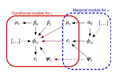
The QALYs and cost distributions are represented in terms of combined modules, the blue and the red boxes, in which the random quantities are linked through logical relationships. This ensures the full characterisation of the uncertainty for each variable in the model. Notably, this is general enough to be extended to any suitable distributional assumption, as well as to handle covariates in either or both the modules.

The proposed framework allows jointly tackling of the different complexities that affect the data in a relatively easy way by means of its modular structure and flexible choice for the distributions of the QALYs and cost variables. Using the MenSS trial as motivating example, we start from the original analysis and expand the model using alternative specifications that progressively account for an increasing number of complexities in the outcomes. We specifically focus on appropriately modelling spikes at the boundary and missingness, as they have substantial implications in terms of inferences and, crucially, cost-effectiveness results.

Example

Three model specifications are considered and applied to QALY data from a RCT case study: 1) Normal marginal for the QALYs and Normal conditional for the costs (which is identical to a Bivariate Normal distribution for the two outcomes); 2) Beta marginal for the QALYs and Gamma conditional for the costs; and 3) Hurdle Model. The following Figure shows the observed QALYs in both treatment groups (indicated with black crosses) as well as summaries of the posterior distributions for the imputed values, obtained from each model. Imputations are distinguished based on whether the corresponding baseline utility value is observed or missing (blue or red lines and dots, respectively) and are summarised in terms of posterior mean and $90%$ HPD intervals.

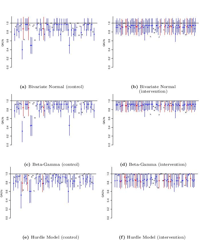
There are clear differences in the imputed values and corresponding credible intervals between the three models in both treatment groups. Neither the Bivariate Normal nor the Beta-Gamma models produce imputed values that capture the structural one component in the data. In addition, as to be expected, the Bivariate Normal fails to respect the natural support for the observed QALYs, with many of the imputations exceeding the unit threshold bound. These unrealistic imputed values highlight the inadequacy of the Normal distribution for the data and may lead to distorted inferences. Conversely, imputations under the Hurdle Model are more realistic, as they can replicate values in the whole range of the observed data, including the structural ones. Imputed unit QALYs with no discernible interval are only observed in the intervention group due to the original data composition, i.e. individuals associated with a unit baseline utility and missing QALYs are almost exclusively present in the intervention group.

Conclusions

We have presented a flexible Bayesian framework that can handle the typical complexities affecting outcome data in CEA, while also being relatively easy to implement using freely available Bayesian software. This is a key advantage that can encourage practitioners to move away from likely biased methods and promote the use of our framework in routine analyses. In conclusion, the proposed framework can:

• Jointly model costs and QALYs;
• Account for skewness and structural values;
• Assess the robustness of the results under a set of differing missingness assumptions.

The original contribution of this work consists in the joint implementation of methods that account for the complexities of the data within a unique and flexible framework that is relatively easy to apply. In the next chapter we will take a step forward in the analysis and present a longitudinal model that can use all observed utility and cost data in the analysis, explore alternative nonignorable missing data assumptions, while simultaneously handling the complexities that affect the data.