Introduction

Economic evaluation alongside Randomised Clinical Trials (RCTs) is an important and increasingly popular component of the process of technology appraisal. The typical analysis of individual level data involves the comparison of two interventions for which suitable measures of clinical benefits and costs are observed on each patient enrolled in the trial at different time points throughout the follow up. Individual level data from RCTs are almost invariably affected by missingness. The recorded outcome process is often incomplete due to individuals who drop out or are observed intermittently throughout the study, causing some observations to be missing. In most applications, the economic evaluation is performed on the cross-sectional variables, computed using only the data from the individuals who are observed at each time point in the trial (completers), with at most limited sensitivity analysis to missingness assumptions. This, however, is an extremely inefficient approach as the information from the responses of all partially observed subjects is completely lost and it is also likely biased unless the completers are a random sample of the subjects on each arm. The problem of missingness is often embedded within a more complex framework, which makes the modelling task in economic evaluations particularly challenging. Specifically, the effectiveness and cost data typically present a series of complexities that need to be simultaneously addressed to avoid biased results.

Using a recent randomised trial as our motivating example, we present a Bayesian parametric model for conducting inference on a bivariate health economic longitudinal response. We specify our model to account for the different types of complexities affecting the data while accommodating a sensitivity analysis to explore the impact of alternative missingness assumptions on the inferences and on the decision-making process for health technology assessment.

Standard approach

To perform the economic evaluation, aggregated measures for both utilities and costs are typically derived from the longitudinal responses recorded in the study. QALYs ($e_{it}$) and total costs ($c_{it}$) measures are computed as:

\[ e_{it}=\sum_{j=1}^{J}(u_{ijt}+u_{ij-1t})\frac{\delta_{j}}{2} ;;; \text{and} ;;;\ c_{it}=\sum_{j=1}^{J}c_{ijt}, \]

where $t$ denotes the treatment group, while $\delta_{j}=\frac{\text{Time}_{j}-\text{Time}_{j-1}}{\text{Unit of time}}$ is the percentage of the time unit (typically one year) which is covered between time $j-1$ and $j$ in the trial. The economic evaluation is then performed by applying some parametric model $p(e_{it},c_{it}\mid \boldsymbol \theta)$, indexed by a set of parameters $\boldsymbol \theta$, to these cross-sectional quantities, typically using linear regression methods to account for the imbalance in some baseline variables between treatments. We note that the term cross-sectional here refers to analyses based on variables derived from the combination of repeated measurements collected at different times over the trial duration and not on data collected at a single point in time. Finally, QALYs and total costs population mean values are derived from the model:

\[ \mu_{et} = \text{E}\left(e_{it} \mid \boldsymbol \theta\right) ;;; \text{and} ;;; \mu_{ct} = \text{E}\left(c_{it} \mid \boldsymbol \theta \right). \]

The differences in $\mu_{et}$ and $\mu_{ct}$ between the treatment groups represent the quantities of interest in the economic evaluation and are used in assessing the relative cost-effectiveness of the interventions. This modelling approach has the limitation that $\mu_{et}$ and $\mu_{ct}$ are derived based only on the completers in the study and does not assess the robustness of the results to a range of plausible missingness assumptions. The model also fails to account for the different complexities that affect the utility and cost data in the trial: from the correlation between variables to the skewness and the presence of structural values (zero for the costs and one for the utilities) in both outcomes.

Longitudinal model to deal with missingness

We propose an alternative approach to deal with a missing bivariate outcome in economic evaluations, while simultaneously allowing for the different complexities that typically affect utility and cost data. Our approach includes a longitudinal model that improves the current practice by taking into account the information from all observed data as well as the time dependence between the responses.

Let $\boldsymbol u_i=(u_{i0},\ldots,u_{iJ})$ and $\boldsymbol c_i=(c_{i0},\ldots,c_{iJ})$ denote the vectors of utilities and costs that were supposed to be observed for subject $i$ at time $j$ in the study, with $j \in {0,1,J}$. We denote with $\boldsymbol y_{ij}=(u_{ij},c_{ij})$ the bivariate outcome for subject $i$ formed by the utility and cost pair at time $j$. We group the individuals according to the missingness patterns and denote with $\boldsymbol r_{ij}=(r^u_{ij},r^c_{ij})$ a pair of indicator variables that take value $1$ if the corresponding outcome for subject $i$ at time $j$ is observed and $0$ otherwise. We denote with $\boldsymbol r_i = (\boldsymbol r_{i0}, \ldots, \boldsymbol r_{iJ})$ the missingness pattern to which subject $i$ belongs, where each pattern is associated with different values for $\boldsymbol r_{ij}$.

We then define our modelling strategy and factor the joint distribution for the response and missingness as:

\[ p(\boldsymbol y, \boldsymbol r \mid \boldsymbol \omega) = p(\boldsymbol y^{\boldsymbol r}_{obs}, \boldsymbol r \mid \boldsymbol \omega)p(\boldsymbol y^{\boldsymbol r}_{mis} \mid \boldsymbol y^{\boldsymbol r}_{obs}, \boldsymbol r, \boldsymbol \omega) \]

where $\boldsymbol y^{\boldsymbol r}_{obs}$ and $\boldsymbol y^{\boldsymbol r}_{mis}$ indicate the observed and missing responses within pattern $\boldsymbol r$, respectively. This is the extrapolation factorisation and factors the joint into two components, of which the extrapolation distribution $p(\boldsymbol y^{\boldsymbol r}_{mis} \mid \boldsymbol y^{\boldsymbol r}_{obs}, \boldsymbol r, \boldsymbol \omega)$ remains unidentified by the data in the absence of unverifiable assumptions about the full data.

To specify the observed data distribution $p(\boldsymbol y^{\boldsymbol r}_{obs}, \boldsymbol r \mid \boldsymbol \omega)$ we use a working model $p^{\star}$ for the joint distribution of the response and missingness. Essentially, the idea is to use the working model $p^{\star}(\boldsymbol y, \boldsymbol{r} \mid \boldsymbol \omega)$ to draw inferences about the distribution of the observed data $p(\boldsymbol y^{\boldsymbol r}_{obs}, \boldsymbol r \mid \boldsymbol \omega)$ by integrating out the missing responses:

\[ p(\boldsymbol y^{\boldsymbol r}_{obs}, \boldsymbol r \mid \boldsymbol \omega) = \int p^{\star}(\boldsymbol y, \boldsymbol{r} \mid \boldsymbol \omega)d \boldsymbol y^{\boldsymbol r}_{mis}. \]

This approach avoids direct specification of the joint distribution of the observed and missing data $p(\boldsymbol y, \boldsymbol r\mid \boldsymbol \omega)$, which has the undesirable consequence of identifying the extrapolation distribution with assumptions that are difficult to check. Indeed, since we use $p^{\star}(\boldsymbol y, \boldsymbol r \mid \boldsymbol \omega)$ only to obtain a model for $p(\boldsymbol y^{\boldsymbol r}_{obs}, \boldsymbol r \mid \boldsymbol \omega)$ and not as a basis for inference, the extrapolation distribution is left unidentified. Any inference depending on the observed data distribution may be obtained using the working model as the true model, with the advantage that it is often easier to specify a model for the the full data $p(\boldsymbol y,\boldsymbol r)$ compared with a model for the observed data $p(\boldsymbol y^{\boldsymbol r}_{obs},\boldsymbol r)$.

We specify $p^{\star}$ using a pattern mixture approach, factoring the joint $p(\boldsymbol y,\boldsymbol r \mid \boldsymbol \omega)$ as the product between the marginal distribution of the missingness patterns $p(\boldsymbol r\mid \boldsymbol \psi)$ and the distribution of the response conditional on the patterns $p(\boldsymbol y\mid \boldsymbol r,\boldsymbol \theta)$, respectively indexed by the distinct parameter vectors $\boldsymbol \psi$ and $\boldsymbol \theta$. If missingness is monotone it is possible to summarise the patterns by dropout time and directly model the dropout process. Unfortunately, as it often occurs in trial-based health economic data, missingness in the case study is mostly nonmonotone and the sparsity of the data in most patterns makes it infeasible to fit the response model within each pattern, with the exception of the completers ($\boldsymbol r = \boldsymbol 1$). Thus, we decided to collapse together all the non-completers patterns ($\boldsymbol r \neq \boldsymbol 1$) and fit the model separately to this aggregated pattern and to the completers. The joint distribution has three components. The first is given by the model for the patterns and the model for the completers ($\boldsymbol r = \boldsymbol 1$), where no missingness occurs. The second component is a model for the observed data in the collapsed patterns $\boldsymbol r \neq \boldsymbol 1$ that, together with the first component, form the observed data distribution. The last component is the extrapolation distribution.

Because the targeted quantities of interest can be derived based on the marginal utility and cost means at each time $j$, in our analysis we do not require the full identification of $p(\boldsymbol y^{\boldsymbol r}_{mis} \mid \boldsymbol y^{\boldsymbol r}_{obs}, \boldsymbol r,\boldsymbol \xi)$. Instead, we only partially identify the extrapolation distribution using partial identifying restrictions. Specifically, we only require the identification of the marginal means for the missing responses in each pattern. We identify the marginal mean of $\boldsymbol y^{\boldsymbol r}_{mis}$ using the observed values, averaged across $\boldsymbol r^\prime \neq \boldsymbol 1$, and some sensitivity parameters $\boldsymbol \Delta = (\Delta_u,\Delta_c)$. Therefore, we compute the marginal means by averaging only across the observed components in pattern ${\boldsymbol r}^\prime$ and ignore the components that are missing.

We start by setting a benchmark assumption with $\boldsymbol \Delta = \boldsymbol 0$, and then explore the sensitivity of the results to alternative scenarios by using different prior distributions on $\boldsymbol \Delta$, calibrated on the observed data. This provides a convenient benchmark scenario from which departures can be explored using alternative informative priors on $\boldsymbol \Delta$. Once the working model has been fitted to the observed data and the extrapolation distribution has been identified, the overall marginal mean for the response model can be computed by marginalising over $\boldsymbol r$, i.e. $\text{E}\left[\boldsymbol Y\right] = \sum_{\boldsymbol r} p(\boldsymbol r)\text{E}\left[\boldsymbol Y \mid \boldsymbol r \right]$.

Modelling framework

The distribution of the observed responses $\boldsymbol y_{ijt}=(u_{ijv},c_{ijt})$ is specified in terms of a model for the utility and cost variables at time $j=0,1,2$, which are jointly modelled without using a multilevel approach and separately by treatment group. In particular, the joint distribution for $\boldsymbol y_{ijt}$ is specified as a series of conditional distributions that capture the dependence between utilities and costs as well as the time dependence.

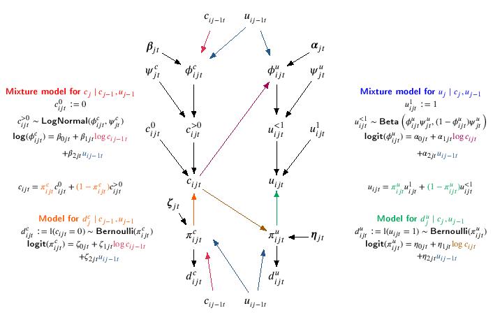
Following the recommendations from the published literature, we account for the skewness using Beta and Log-Normal distributions for the utilities and costs, respectively. Since the Beta distribution does not allow for negative values, we scaled the utilities on $[0,1]$ through the transformation $u^{\star}_{ij}=\frac{u_{ij}-\text{min}(\boldsymbol u_{j})}{\text{max}(\boldsymbol u_{j})-\text{min}(\boldsymbol u_{j})}$, and fit the model to these transformed variables. To account for the structural values $u_{ij} = 1$ and $c_{ij} = 0$ we use a hurdle approach by including in the model the indicator variables $d^u_{ij}:=\mathbb{I}(u_{ij}=1)$ and $d^c_{ij}:=\mathbb{I}(c_{ij}=0)$, which take value $1$ if subject $i$ is associated with a structural value at time $j$ and 0 otherwise. The probabilities of observing these values, as well as the mean of each variable, are then modelled conditionally on other variables via linear regressions defined on the logit or log scale. Specifically, at time $j=1,2$, the probability of observing a zero and the mean costs are modelled conditionally on the utilities and costs at the previous times, while the probability of observing a one and the mean utilities are modelled conditionally on the current costs (also at $j=0$) and the utilities at the previous times (only at $j=1,2$). The model is summarised by the following Figure.

We use partial identifying restrictions to link the observed data distribution $p(\boldsymbol y_{obs},\boldsymbol r)$ to the extrapolation distribution $p(\boldsymbol y_{mis} \mid \boldsymbol y_{obs},\boldsymbol r)$ and consider interpretable deviations from a benchmark scenario to assess how inferences are driven by our assumptions. Specifically, we identify the marginal mean of the missing responses in each pattern $\boldsymbol y^{\boldsymbol r}_{mis}$ by averaging across the corresponding components that are observed and add the sensitivity parameters $\boldsymbol \Delta_j$.

We define $\boldsymbol \Delta_j=(\Delta_{c_{j}},\Delta_{u_{j}})$ to be time-specific location shifts at the marginal mean in each pattern and set $\boldsymbol \Delta_j = \boldsymbol 0$ as the benchmark scenario. We then explore departures from this benchmark using alternative priors on $\boldsymbol \Delta_j$, which are calibrated using the observed standard deviations for costs and utilities at each time $j$ to define the amplitude of the departures from $\boldsymbol \Delta_j=\boldsymbol 0$.

Conlcusions

Missingness represents a threat to economic evaluations as, when dealing with partially-observed data, any analysis makes assumptions about the missing values that cannot be verified from the data at hand. Trial-based analyses are typically conducted on cross-sectional quantities, e.g. QALYs and total costs, which are derived based only on the observed data from the completers in the study. This is an inefficient approach which may discard a substantial proportion of the sample, especially when there is a relatively large number of time points, where individuals are more likely to have some missing value or to drop out from the study. In addition, when there are systematic differences between the responses of the completers and non-completers, which is typically the case when dealing with self-reported outcomes in trial-based analyses, the results based only on the former may be biased and mislead the final assessment. A further concern is that routine analyses typically rely on standard models that ignore or at best fail to properly account for potentially important features in the data such as correlation, skewness, and the presence of structural values.

Our framework represents a considerable step forward for the handling of missingness in economic evaluations compared with the current practice, which typically relies on methods that assume an ignorable MAR and rarely conducts sensitivity analysis to MNAR departures. Nevertheless, further improvements are certainly possible. For example, a potential area for future work is to increase the flexibility of our approach through a semi-parametric or nonparametric specification for the observed data distribution, which would allow a weakening of the model assumptions and likely further improve the fit of the model to the observed data and address sparse patterns in an automated way. As for the extrapolation distribution, alternative identifying restrictions that introduce the sensitivity parameters via the conditional mean (rather than the marginal mean) could be considered, and their impact on the conclusions assessed in a sensitivity analysis.