Modelling Framework

We extend and adapt the modelling frameworks typically used for the analysis of football data and propose a novel Bayesian hierarchical modelling framework for the analysis and prediction of volleyball results in regular seasons. Three different sub-models or “modules” form our framework: (1) The module of the observed number of points scored by the two opposing teams in a match ($y_h$ and $y_a$); (2) the module of the binary indicator for the number of sets played ($d^s$); (3) the module of the binary indicator for the winner of the match ($d^m$). These three modules are jointly modelled using a flexible Bayesian parametric approach, which allows to fully propagate the uncertainty for each unobserved quantity and to assess the predictive performance of the model in a relatively easy way. In the following, we describe the notation and the model used in each of the three modules.

Module 1: Modelling the Scoring Intensity

In the first module of the framework, we model the number of points scored by the home and away team in the $i$-th match of the season $\boldsymbol y=(y_{hi},y_{ai})$ using two independent Poisson distributions

\[ y_{hi} \sim Poisson(\theta_{hi}), \]

\[ y_{ai} \sim Poisson(\theta_{ai}), \]

conditionally on the set of parameters $\boldsymbol \theta=(\theta_{hi},\theta_{ai})$, representing the scoring intensity in the $i$-th match for the home and away team, respectively. These parameters are then modelled using the log-linear regressions

\[ log(\theta_{hi}) =\mu + \lambda + att_{h(i)} + def_{a(i)}, \]

\[ log(\theta_{ai}) =\mu + att_{a(i)} + def_{h(i)}, \]

which corresponds to a Poisson log-linear model. Within these formulae, $\mu$ is a constant, while $\lambda$ can be identified as the home effect and represents the advantage for the team hosting the game which is typically assumed to be constant for all the teams and throughout the season. The overall offensive and defensive performances of the $k$-th team is captured by the parameters $att$ and $def$, whose nested indexes $h(i), a(i)=1,\ldots,K$ identify the home and away team in the $i$-th game of the season, where $K$ denotes the total number of the teams.

We then expand the modelling framework to incorporate match-specific statistics related to the offensive and defensive performances of the home and away teams. More specifically, the effects associated with the attack intensity of the home teams and the defence effect of the away teams are:

\[ att_{h(i)} =\alpha_{0h(i)} + \alpha_{1h(i)}att^{eff}_{hi} + \alpha_{2h(i)}ser^{eff}_{hi}, \]

\[ def_{a(i)} =\beta_{0a(i)} + \beta_{1a(i)}def^{eff}_{ai} + \beta_{2a(i)}blo^{eff}_{ai}. \]

We omit the index $i$ from the terms to the left-hand side of the above formulae to ease notation, i.e. $att_{h(i)}=att_{h(i)i}$ and $def_{a(i)}=def_{a(i)i}$. The overall offensive effect of the home teams is a function of a baseline team specific parameter $\alpha_{0h(i)}$, and the attack and serve efficiencies of the home team, whose impact is captured by the parameters $\alpha_{1h(i)}$ and $\alpha_{2h(i)}$. The overall defensive effect of the away team is a function of a baseline team-specific parameter $\beta_{0a(i)}$, and the defence and block efficiencies of the away team, whose impact is captured by the parameters $\beta_{1a(i)}$ and $\beta_{2a(i)}$, respectively. Similarly, the effects associated with the attack intensity of the away teams and the defence effect of the home teams are:

\[ att_{a(i)} =\alpha_{0a(i)} + \alpha_{1a(i)}att^{eff}_{ai}+ \alpha_{2a(i)}ser^{eff}_{ai}, \]

\[ def_{h(i)} =\beta_{0h(i)} + \beta_{1h(i)}def^{eff}_{hi}+ \beta_{2h(i)}blo^{eff}_{hi}, \]

To achieve identifiability of the model, a set of parametric constraints needs to be imposed. We impose sum-to-zero constraints on the team-specific parameters, i.e. we set $\sum_{k=1}^{K}\alpha_{jk}=0$ and $\sum_{k=1}^{K}\beta_{jk}=0$, for $k=1,\ldots,K$ and $j=(0,1,2)$. Under this set of constraints, the overall offensive and defensive effects of the teams are expressed as departures from a team of average offensive and defensive performance. Within a Bayesian framework, prior distributions need to be specified for all random parameters in the model. Weakly informative Normal distributions centred at $0$ with a relatively large variances are specified for the fixed effect parameters.

Module 2: Modelling the Probability of Playing 5 Sets

In the second module, we explicitly model the chance of playing $5$ sets in the $i$-th match of the season, i.e. the sum of the sets won by the home ($s_{hi}$) and away ($s_{ai}$) team is equal to $5$. This is necessary when generating predictions in order to correctly assign the points to the winning/losing teams throughout the season and evaluate the rankings of the teams at the end of the season. We model the indicator variable $d^s_{i}$, taking value $1$ if $5$ sets were played in the $i-$th match and $0$ otherwise, using a Bernoulli distribution

\[ d^s_{i}:=\mathbb{I}(s_{hi}+s_{ai}=5)\sim\mbox{Bernoulli}(\pi^s_{i}), \]

where

\[ logit(\pi^s_{i})= \gamma_0 + \gamma_1y_{hi} + \gamma_2y_{ai}.
\]

Module 3: Modelling the Probability of Winning the Match

The last module deals with the chance of the home team to win the $i$-th match, i.e. the total number of sets won by the home team ($s_{hi}$) is larger than that of the away team ($s_{ai}$) – we note that we could have also equivalently decided to model the chance of the away team to win the $i$-th match. This part of the model is again necessary when predicting the results for future matches, since the team associated with the higher number of points scored in the $i$-th match may not correspond to the winning team. We model the indicator variable $d^m_{i}$, taking value $1$ if the home team won the $i-$th match and $0$ otherwise, using another Bernoulli distribution

\[ d^m_{i}:=\mathbb{I}(s_{hi}>s_{ai}) \sim\mbox{Bernoulli}(\pi^m_{i}), \]

where

\[ logit(\pi^m_{i})= \eta_0 + \eta_1y_{hi} + \eta_2y_{ai} + \eta_3 d^s_i. \]

The next figure shows a graphical representation of the modelling framework proposed.

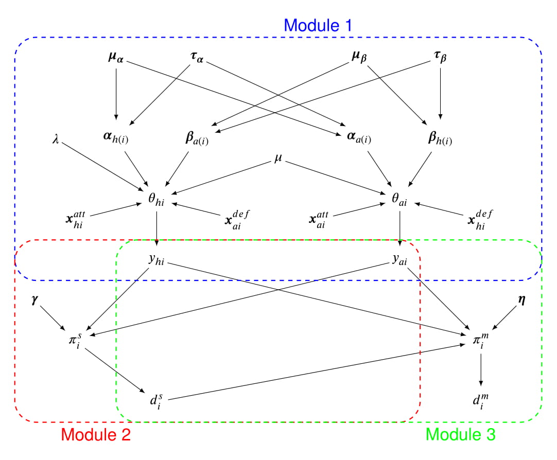
The framework corresponds to a joint distribution for all the observed quantities which are explicitly modelled. This is factored into the product of the marginal distribution of the total number of points scored by the two teams in each match, Module 1 – $p(\boldsymbol y)$, the conditional distribution of the probability of playing $5$ sets in a match given $\boldsymbol y$, Module 2 – $p(d^s_i \mid \boldsymbol y)$, and the conditional probability of winning the match given $\boldsymbol y$ and $d^s_i$, Module 3 – $p(d^m_i\mid \boldsymbol y, d^s_i)$. Module 1 also includes the different in-game statistics as covariates in the model. These are related to the either the offensive (serve and attack efficiency) or defensive (defence and block efficiency) effects of the home and away teams in each match of the season, and are respectively denoted in the graph as $\boldsymbol x^{att}_{ti}=(ser^{eff}_{ti}, att^{eff}_{ti})$ and $\boldsymbol x^{def}_{ti}=(def^{eff}_{ti}, blo^{eff}_{ti})$ to ease notation, for $t=(h,a)$.

Accounting for the multilevel correlation

Although the individual-level correlation between the observable variables $y_{hi}$ and $y_{ai}$ is taken into account through the hierarchical structure of the framework, a potential limitation of the model is that it ignores the possible multilevel correlation between the team-specific offensive $\alpha_{jk}$ and defensive $\beta_{jk}$ coefficients, for $j=(0,1,2)$ and $k=1,\ldots,K$. In an alternative analysis, we account for the multilevel correlation using Inverse-Wishart distributions on the covariance matrix of the team specific parameters $ \boldsymbol \Sigma_{\boldsymbol \alpha}$ and $ \boldsymbol \Sigma_{\boldsymbol \beta}$, which are scaled in order to facilitate the specification of the priors.

Results

Overall, the predicted results from both the basic and the scaled IW model seem to replicate the observed data relatively well for most of the teams. The total number of points scored and conceded are similar between the observed and replicated data, with the teams scoring (conceding) the most being also associated with the highest replicated points scored (conceded) and vice versa. Relatively small discrepancies are observed between the results of the two models for some of the teams. The total number of wins and league points are almost identical between the observed and replicated data, with the scaled IW model being associated with slightly m ore accurate predictions compared with the basic model.

The following figure compares the cumulative points derived from the observed results throughout the season (the black line) and the predictions from both the basic model (in red), and the scaled Inverse-Wishart model (in blue).

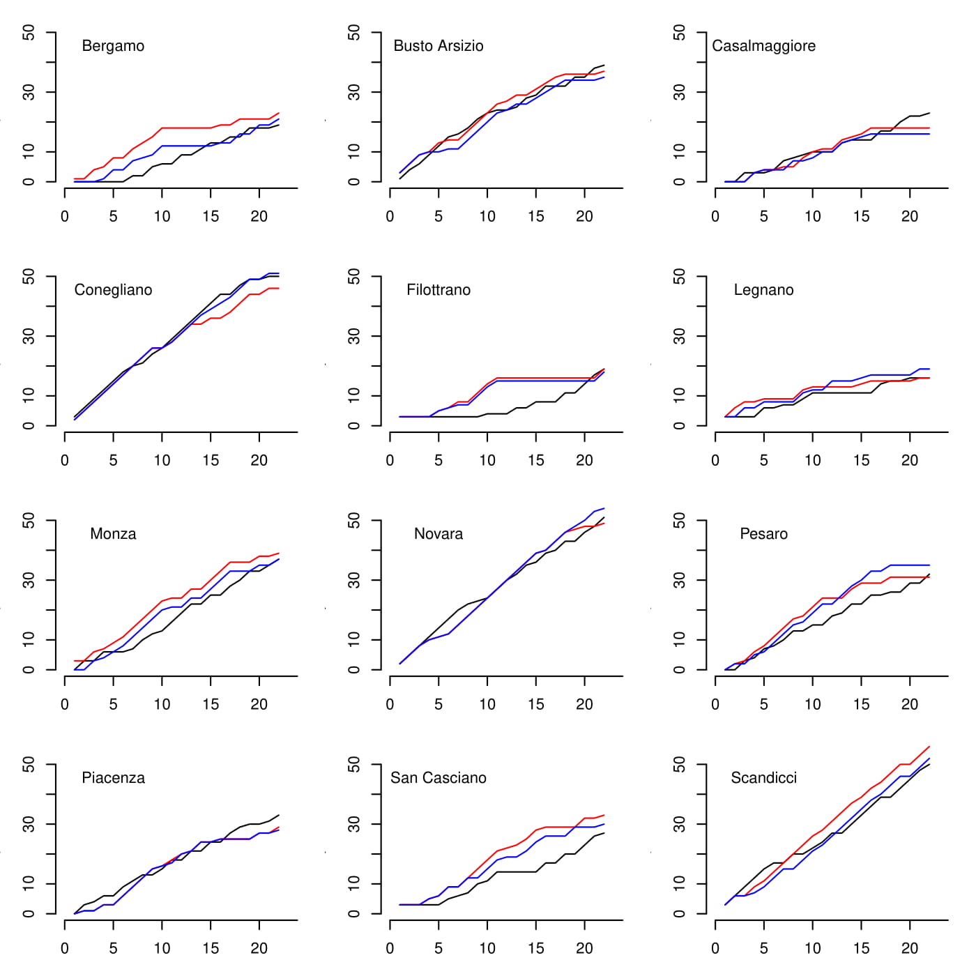
For almost all teams the predicted results are relatively close to the observed data and suggest a good performance of both models.

Conclusions

To our knowledge, this is the first modelling framework which jointly allows to predict team rankings and the outcomes of the matches during a season in volleyball. The two alternative specifications implemented in our analysis show generally good predictive performances; between the two models, the scaled IW model seems to be slightly more accurate compared with the basic model, but is also associated with a higher level of complexity.