Randomised Complete Block Anova - STAN

Feb 10, 2020 R, anova, STAN, randomised complete block

This tutorial will focus on the use of Bayesian estimation to fit simple linear regression models. BUGS (Bayesian inference Using Gibbs Sampling) is an algorithm and supporting language (resembling R) dedicated to performing the Gibbs sampling implementation of Markov Chain Monte Carlo (MCMC) method. Dialects of the BUGS language are implemented within three main projects:

OpenBUGS - written in component pascal.
JAGS - (Just Another Gibbs Sampler) - written in C++.
STAN - a dedicated Bayesian modelling framework written in C++ and implementing Hamiltonian MCMC samplers.

Whilst the above programs can be used stand-alone, they do offer the rich data pre-processing and graphical capabilities of R, and thus, they are best accessed from within R itself. As such there are multiple packages devoted to interfacing with the various software implementations:

R2OpenBUGS - interfaces with OpenBUGS
R2jags - interfaces with JAGS
rstan - interfaces with STAN

This tutorial will demonstrate how to fit models in STAN (Gelman, Lee, and Guo (2015)) using the package rstan (Stan Development Team (2018)) as interface, which also requires to load some other packages.

Overview

Introduction

In the previous tutorial (nested ANOVA), we introduced the concept of employing sub-replicates that are nested within the main treatment levels as a means of absorbing some of the unexplained variability that would otherwise arise from designs in which sampling units are selected from amongst highly heterogeneous conditions. Such (nested) designs are useful in circumstances where the levels of the main treatment (such as burnt and un-burnt sites) occur at a much larger temporal or spatial scale than the experimental/sampling units (e.g. vegetation monitoring quadrats). For circumstances in which the main treatments can be applied (or naturally occur) at the same scale as the sampling units (such as whether a stream rock is enclosed by a fish proof fence or not), an alternative design is available. In this design (randomised complete block design), each of the levels of the main treatment factor are grouped (blocked) together (in space and/or time) and therefore, whilst the conditions between the groups (referred to as “blocks”) might vary substantially, the conditions under which each of the levels of the treatment are tested within any given block are far more homogeneous.

If any differences between blocks (due to the heterogeneity) can account for some of the total variability between the sampling units (thereby reducing the amount of variability that the main treatment(s) failed to explain), then the main test of treatment effects will be more powerful/sensitive. As an simple example of a randomised complete block (RCB) design, consider an investigation into the roles of different organism scales (microbial, macro invertebrate and vertebrate) on the breakdown of leaf debris packs within streams. An experiment could consist of four treatment levels - leaf packs protected by fish-proof mesh, leaf packs protected by fine macro invertebrate exclusion mesh, leaf packs protected by dissolving antibacterial tablets, and leaf packs relatively unprotected as controls. As an acknowledgement that there are many other unmeasured factors that could influence leaf pack breakdown (such as flow velocity, light levels, etc) and that these are likely to vary substantially throughout a stream, the treatments are to be arranged into groups or “blocks” (each containing a single control, microbial, macro invertebrate and fish protected leaf pack). Blocks of treatment sets are then secured in locations haphazardly selected throughout a particular reach of stream. Importantly, the arrangement of treatments in each block must be randomized to prevent the introduction of some systematic bias - such as light angle, current direction etc.

Blocking does however come at a cost. The blocks absorb both unexplained variability as well as degrees of freedom from the residuals. Consequently, if the amount of the total unexplained variation that is absorbed by the blocks is not sufficiently large enough to offset the reduction in degrees of freedom (which may result from either less than expected heterogeneity, or due to the scale at which the blocks are established being inappropriate to explain much of the variation), for a given number of sampling units (leaf packs), the tests of main treatment effects will suffer power reductions. Treatments can also be applied sequentially or repeatedly at the scale of the entire block, such that at any single time, only a single treatment level is being applied (see the lower two sub-figures above). Such designs are called repeated measures. A repeated measures ANOVA is to an single factor ANOVA as a paired t-test is to a independent samples t-test. One example of a repeated measures analysis might be an investigation into the effects of a five different diet drugs (four doses and a placebo) on the food intake of lab rats. Each of the rats (“subjects”) is subject to each of the four drugs (within subject effects) which are administered in a random order. In another example, temporal recovery responses of sharks to bi-catch entanglement stresses might be simulated by analyzing blood samples collected from captive sharks (subjects) every half hour for three hours following a stress inducing restraint. This repeated measures design allows the anticipated variability in stress tolerances between individual sharks to be accounted for in the analysis (so as to permit more powerful test of the main treatments). Furthermore, by performing repeated measures on the same subjects, repeated measures designs reduce the number of subjects required for the investigation. Essentially, this is a randomised complete block design except that the within subject (block) effect (e.g. time since stress exposure) cannot be randomised.

To suppress contamination effects resulting from the proximity of treatment sampling units within a block, units should be adequately spaced in time and space. For example, the leaf packs should not be so close to one another that the control packs are effected by the antibacterial tablets and there should be sufficient recovery time between subsequent drug administrations. In addition, the order or arrangement of treatments within the blocks must be randomized so as to prevent both confounding as well as computational complications. Whilst this is relatively straight forward for the classic randomized complete block design (such as the leaf packs in streams), it is logically not possible for repeated measures designs. Blocking factors are typically random factors that represent all the possible blocks that could be selected. As such, no individual block can truly be replicated. Randomised complete block and repeated measures designs can therefore also be thought of as un-replicated factorial designs in which there are two or more factors but that the interactions between the blocks and all the within block factors are not replicated.

Linear models

The linear models for two and three factor nested design are:

\[ y_{ij} = \mu + \beta_i + \alpha_j + \epsilon_{ij},\]

\[ y_{ijk} = \mu + \beta_i + \alpha_j + \gamma_k + (\beta\alpha)_{ij} + (\beta\gamma)_{ik} + (\alpha\gamma)_{jk} + (\alpha\beta\gamma)_{ijk} + \epsilon_{ijk}, \;\;\; \text{(Model 1)}\]

\[ y_{ijk} = \mu + \beta_i + \alpha_j + \gamma_k + (\alpha\gamma)_{jk} + \epsilon_{ijk}, \;\;\; \text{(Model 2)},\]

where \(\mu\) is the overall mean, \(\beta\) is the effect of the Blocking Factor B (\(\sum \beta=0\)), \(\alpha\) and \(\gamma\) are the effects of withing block Factor A and Factor C, respectively, and \(\epsilon \sim N(0,\sigma^2)\) is the random unexplained or residual component.

Tests for the effects of blocks as well as effects within blocks assume that there are no interactions between blocks and the within block effects. That is, it is assumed that any effects are of similar nature within each of the blocks. Whilst this assumption may well hold for experiments that are able to consciously set the scale over which the blocking units are arranged, when designs utilize arbitrary or naturally occurring blocking units, the magnitude and even polarity of the main effects are likely to vary substantially between the blocks. The preferred (non-additive or “Model 1”) approach to un-replicated factorial analysis of some bio-statisticians is to include the block by within subject effect interactions (e.g. \(\beta\alpha\)). Whilst these interaction effects cannot be formally tested, they can be used as the denominators in F-ratio calculations of their respective main effects tests. Proponents argue that since these blocking interactions cannot be formally tested, there is no sound inferential basis for using these error terms separately. Alternatively, models can be fitted additively (“Model 2”) whereby all the block by within subject effect interactions are pooled into a single residual term (\(\epsilon\)). Although the latter approach is simpler, each of the within subject effects tests do assume that there are no interactions involving the blocks and that perhaps even more restrictively, that sphericity holds across the entire design.

Assumptions

As with other ANOVA designs, the reliability of hypothesis tests is dependent on the residuals being:

normally distributed. Boxplots using the appropriate scale of replication (reflecting the appropriate residuals/F-ratio denominator should be used to explore normality. Scale transformations are often useful.
equally varied. Boxplots and plots of means against variance (using the appropriate scale of replication) should be used to explore the spread of values. Residual plots should reveal no patterns. Scale transformations are often useful.
independent of one another. Although the observations within a block may not strictly be independent, provided the treatments are applied or ordered randomly within each block or subject, within block proximity effects on the residuals should be random across all blocks and thus the residuals should still be independent of one another. Nevertheless, it is important that experimental units within blocks are adequately spaced in space and time so as to suppress contamination or carryover effects.

Simple RCB

Data generation

Imagine we has designed an experiment in which we intend to measure a response (y) to one of treatments (three levels; “a1”, “a2” and “a3”). Unfortunately, the system that we intend to sample is spatially heterogeneous and thus will add a great deal of noise to the data that will make it difficult to detect a signal (impact of treatment). Thus in an attempt to constrain this variability you decide to apply a design (RCB) in which each of the treatments within each of 35 blocks dispersed randomly throughout the landscape. As this section is mainly about the generation of artificial data (and not specifically about what to do with the data), understanding the actual details are optional and can be safely skipped.

> library(plyr)
> set.seed(123)
> nTreat <- 3
> nBlock <- 35
> sigma <- 5
> sigma.block <- 12
> n <- nBlock*nTreat
> Block <- gl(nBlock, k=1)
> A <- gl(nTreat,k=1)
> dt <- expand.grid(A=A,Block=Block)
> #Xmat <- model.matrix(~Block + A + Block:A, data=dt)
> Xmat <- model.matrix(~-1+Block + A, data=dt)
> block.effects <- rnorm(n = nBlock, mean = 40, sd = sigma.block)
> A.effects <- c(30,40)
> all.effects <- c(block.effects,A.effects)
> lin.pred <- Xmat %*% all.effects
> 
> # OR
> Xmat <- cbind(model.matrix(~-1+Block,data=dt),model.matrix(~-1+A,data=dt))
> ## Sum to zero block effects
> block.effects <- rnorm(n = nBlock, mean = 0, sd = sigma.block)
> A.effects <- c(40,70,80)
> all.effects <- c(block.effects,A.effects)
> lin.pred <- Xmat %*% all.effects
> 
> 
> 
> ## the quadrat observations (within sites) are drawn from
> ## normal distributions with means according to the site means
> ## and standard deviations of 5
> y <- rnorm(n,lin.pred,sigma)
> data.rcb <- data.frame(y=y, expand.grid(A=A, Block=Block))
> head(data.rcb)  #print out the first six rows of the data set
         y A Block
1 45.80853 1     1
2 66.71784 2     1
3 93.29238 3     1
4 43.10101 1     2
5 73.20697 2     2
6 91.77487 3     2

Exploratory data analysis

Normality and Homogeneity of variance

> boxplot(y~A, data.rcb)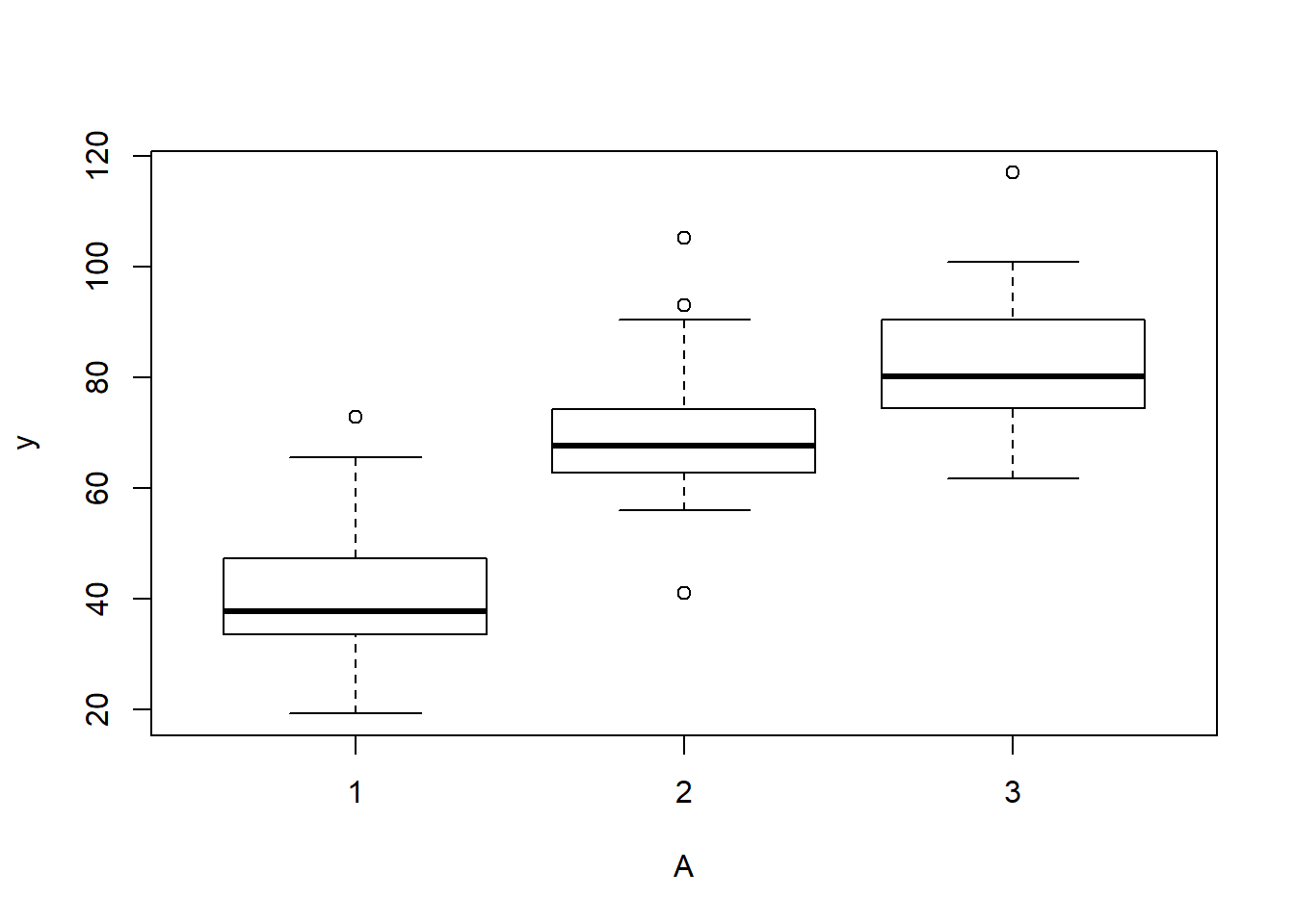

Conclusions:

there is no evidence that the response variable is consistently non-normal across all populations - each boxplot is approximately symmetrical.
there is no evidence that variance (as estimated by the height of the boxplots) differs between the five populations. . More importantly, there is no evidence of a relationship between mean and variance - the height of boxplots does not increase with increasing position along the \(y\)-axis. Hence it there is no evidence of non-homogeneity

Obvious violations could be addressed either by:

transform the scale of the response variables (to address normality, etc). Note transformations should be applied to the entire response variable (not just those populations that are skewed).

Block by within-Block interaction

> library(car)
> with(data.rcb, interaction.plot(A,Block,y))
> 
> #OR with ggplot
> library(ggplot2)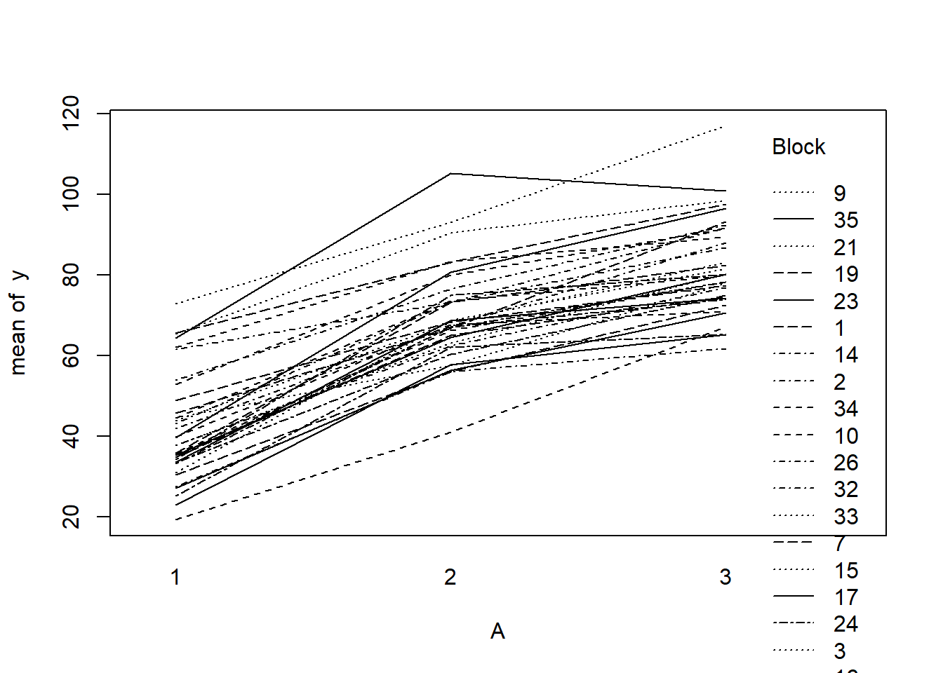

> ggplot(data.rcb, aes(y=y, x=A, group=Block,color=Block)) + geom_line() +
+   guides(color=guide_legend(ncol=3))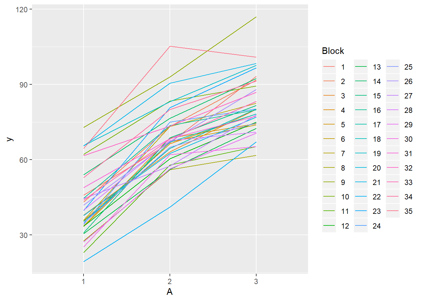

> 
> residualPlots(lm(y~Block+A, data.rcb))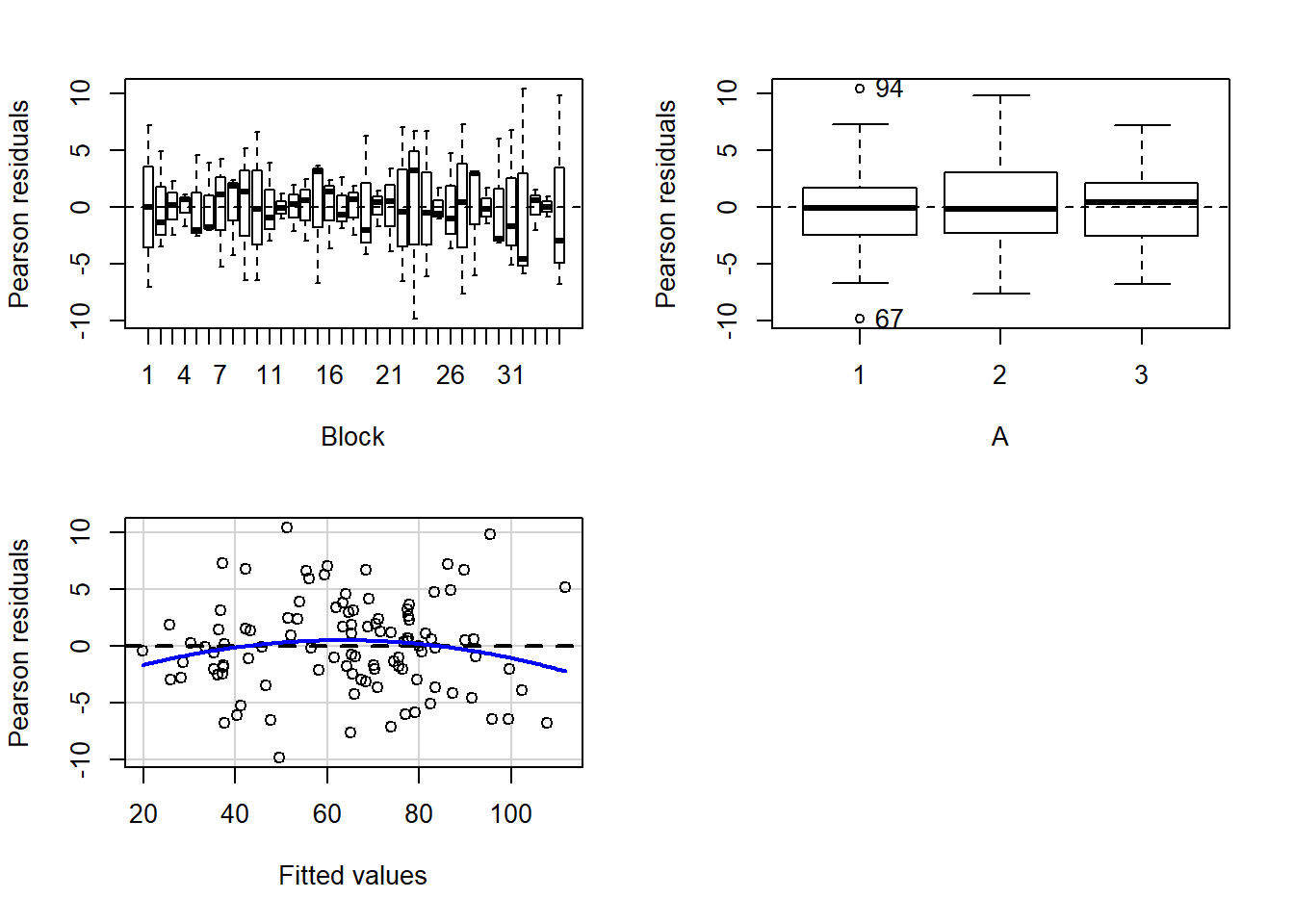

           Test stat Pr(>|Test stat|)
Block                                
A                                    
Tukey test   -1.4163           0.1567
> 
> # the Tukey's non-additivity test by itself can be obtained via an internal function
> # within the car package
> car:::tukeyNonaddTest(lm(y~Block+A, data.rcb))
      Test     Pvalue 
-1.4163343  0.1566776 
> 
> # alternatively, there is also a Tukey's non-additivity test within the
> # asbio package
> library(asbio)
> with(data.rcb,tukey.add.test(y,A,Block))

Tukey's one df test for additivity 
F = 2.0060029   Denom df = 67    p-value = 0.1613102

Conclusions:

there is no visual or inferential evidence of any major interactions between Block and the within-Block effect (A). Any trends appear to be reasonably consistent between Blocks.

Model fitting

Full parameterisation

\[ y_{ijk} \sim N(\mu_{ij}, \sigma^2), \;\;\; \mu_{ij}=\beta_0 + \beta_i + \gamma_{j(i)}, \]

where \(\gamma_{ij)} \sim N(0, \sigma^2_B)\), \(\beta_0, \beta_i \sim N(0, 1000000)\), and \(\sigma^2, \sigma^2_B \sim \text{Cauchy(0, 25)}\). The full parameterisation, shows the effects parameterisation in which there is an intercept (\(\beta_0\)) and two treatment effects (\(\beta_i\), where \(i\) is \(1,2\)).

Matrix parameterisation

\[ y_{ijk} \sim N(\mu_{ij}, \sigma^2), \;\;\; \mu_{ij}=\boldsymbol \beta \boldsymbol X + \gamma_{j(i)}, \]

where \(\gamma_{ij} \sim N(0, \sigma^2_B)\), \(\boldsymbol \beta \sim MVN(0, 1000000)\), and \(\sigma^2, \sigma^2_B \sim \text{Cauchy(0, 25)}\). The full parameterisation, shows the effects parameterisation in which there is an intercept (\(\alpha_0\)) and two treatment effects (\(\beta_i\), where \(i\) is \(1,2\)). The matrix parameterisation is a compressed notation, In this parameterisation, there are three alpha parameters (one representing the mean of treatment a1, and the other two representing the treatment effects (differences between a2 and a1 and a3 and a1). In generating priors for each of these three alpha parameters, we could loop through each and define a non-informative normal prior to each (as in the Full parameterisation version). However, it turns out that it is more efficient (in terms of mixing and thus the number of necessary iterations) to define the priors from a multivariate normal distribution. This has as many means as there are parameters to estimate (\(3\)) and a \(3\times3\) matrix of zeros and \(100\) in the diagonals.

\[ \boldsymbol \mu = \begin{bmatrix} 0 \\ 0 \\ 0 \end{bmatrix}, \;\;\; \sigma^2 \sim \begin{bmatrix} 1000000 & 0 & 0 \\ 0 & 1000000 & 0 \\ 0 & 0 & 1000000 \end{bmatrix}. \]

Hierarchical parameterisation

\[ y_{ijk} \sim N(\mu_{ij}, \sigma^2), \;\;\; \mu_{ij}= \beta_0 + \beta_i + \gamma_{j(i)}, \]

where \(\gamma_{ij} \sim N(0, \sigma^2_B)\), \(\beta_0, \beta_i \sim N(0, 1000000)\), and \(\sigma^2, \sigma^2_B \sim \text{Cauchy(0, 25)}\).

Rather than assume a specific variance-covariance structure, just like lme we can incorporate an appropriate structure to account for different dependency/correlation structures in our data. In RCB designs, it is prudent to capture the residuals to allow checks that there are no outstanding dependency issues following model fitting.

Full means parameterisation

> rstanString="
+ data{
+    int n;
+    int nA;
+    int nB;
+    vector [n] y;
+    int A[n];
+    int B[n];
+ }
+ 
+ parameters{
+   real alpha[nA];
+   real<lower=0> sigma;
+   vector [nB] beta;
+   real<lower=0> sigma_B;
+ }
+  
+ model{
+     real mu[n];
+ 
+     // Priors
+     alpha ~ normal( 0 , 100 );
+     beta ~ normal( 0 , sigma_B );
+     sigma_B ~ cauchy( 0 , 25 );
+     sigma ~ cauchy( 0 , 25 );
+     
+     for ( i in 1:n ) {
+         mu[i] = alpha[A[i]] + beta[B[i]];
+     }
+     y ~ normal( mu , sigma );
+ }
+ 
+ "
> 
> ## write the model to a text file
> writeLines(rstanString, con = "fullModel.stan")

Arrange the data as a list (as required by STAN). As input, STAN will need to be supplied with: the response variable, the predictor matrix, the number of predictors, the total number of observed items. This all needs to be contained within a list object. We will create two data lists, one for each of the hypotheses.

> data.rcb.list <- with(data.rcb, list(y=y, A=as.numeric(A), B=as.numeric(Block),
+   n=nrow(data.rcb), nB=length(levels(Block)),nA=length(levels(A))))

Define the nodes (parameters and derivatives) to monitor and the chain parameters.

> params <- c("alpha","sigma","sigma_B")
> burnInSteps = 3000
> nChains = 2
> numSavedSteps = 3000
> thinSteps = 1
> nIter = burnInSteps+ceiling((numSavedSteps * thinSteps)/nChains)

Start the STAN model (check the model, load data into the model, specify the number of chains and compile the model). Load the rstan package.

> library(rstan)

Now run the STAN code via the rstan interface.

> data.rcb.rstan.c <- stan(data = data.rcb.list, file = "fullModel.stan", 
+                          chains = nChains, pars = params, iter = nIter, 
+                          warmup = burnInSteps, thin = thinSteps)

SAMPLING FOR MODEL 'fullModel' NOW (CHAIN 1).
Chain 1: 
Chain 1: Gradient evaluation took 0 seconds
Chain 1: 1000 transitions using 10 leapfrog steps per transition would take 0 seconds.
Chain 1: Adjust your expectations accordingly!
Chain 1: 
Chain 1: 
Chain 1: Iteration:    1 / 4500 [  0%]  (Warmup)
Chain 1: Iteration:  450 / 4500 [ 10%]  (Warmup)
Chain 1: Iteration:  900 / 4500 [ 20%]  (Warmup)
Chain 1: Iteration: 1350 / 4500 [ 30%]  (Warmup)
Chain 1: Iteration: 1800 / 4500 [ 40%]  (Warmup)
Chain 1: Iteration: 2250 / 4500 [ 50%]  (Warmup)
Chain 1: Iteration: 2700 / 4500 [ 60%]  (Warmup)
Chain 1: Iteration: 3001 / 4500 [ 66%]  (Sampling)
Chain 1: Iteration: 3450 / 4500 [ 76%]  (Sampling)
Chain 1: Iteration: 3900 / 4500 [ 86%]  (Sampling)
Chain 1: Iteration: 4350 / 4500 [ 96%]  (Sampling)
Chain 1: Iteration: 4500 / 4500 [100%]  (Sampling)
Chain 1: 
Chain 1:  Elapsed Time: 0.406 seconds (Warm-up)
Chain 1:                0.218 seconds (Sampling)
Chain 1:                0.624 seconds (Total)
Chain 1: 

SAMPLING FOR MODEL 'fullModel' NOW (CHAIN 2).
Chain 2: 
Chain 2: Gradient evaluation took 0 seconds
Chain 2: 1000 transitions using 10 leapfrog steps per transition would take 0 seconds.
Chain 2: Adjust your expectations accordingly!
Chain 2: 
Chain 2: 
Chain 2: Iteration:    1 / 4500 [  0%]  (Warmup)
Chain 2: Iteration:  450 / 4500 [ 10%]  (Warmup)
Chain 2: Iteration:  900 / 4500 [ 20%]  (Warmup)
Chain 2: Iteration: 1350 / 4500 [ 30%]  (Warmup)
Chain 2: Iteration: 1800 / 4500 [ 40%]  (Warmup)
Chain 2: Iteration: 2250 / 4500 [ 50%]  (Warmup)
Chain 2: Iteration: 2700 / 4500 [ 60%]  (Warmup)
Chain 2: Iteration: 3001 / 4500 [ 66%]  (Sampling)
Chain 2: Iteration: 3450 / 4500 [ 76%]  (Sampling)
Chain 2: Iteration: 3900 / 4500 [ 86%]  (Sampling)
Chain 2: Iteration: 4350 / 4500 [ 96%]  (Sampling)
Chain 2: Iteration: 4500 / 4500 [100%]  (Sampling)
Chain 2: 
Chain 2:  Elapsed Time: 0.347 seconds (Warm-up)
Chain 2:                0.187 seconds (Sampling)
Chain 2:                0.534 seconds (Total)
Chain 2: 
> 
> print(data.rcb.rstan.c, par = c("alpha", "sigma", "sigma_B"))
Inference for Stan model: fullModel.
2 chains, each with iter=4500; warmup=3000; thin=1; 
post-warmup draws per chain=1500, total post-warmup draws=3000.

          mean se_mean   sd  2.5%   25%   50%   75% 97.5% n_eff Rhat
alpha[1] 41.62    0.10 2.22 37.25 40.16 41.60 43.04 46.10   503    1
alpha[2] 69.56    0.10 2.23 65.09 68.08 69.55 71.00 74.06   501    1
alpha[3] 81.91    0.10 2.21 77.50 80.46 81.89 83.35 86.41   512    1
sigma     5.06    0.01 0.45  4.28  4.74  5.03  5.35  6.06  2235    1
sigma_B  11.71    0.03 1.53  9.19 10.60 11.57 12.67 15.17  3266    1

Samples were drawn using NUTS(diag_e) at Thu Feb 20 11:13:14 2020.
For each parameter, n_eff is a crude measure of effective sample size,
and Rhat is the potential scale reduction factor on split chains (at 
convergence, Rhat=1).
> 
> data.rcb.rstan.c.df <-as.data.frame(extract(data.rcb.rstan.c))
> head(data.rcb.rstan.c.df)
   alpha.1  alpha.2  alpha.3    sigma   sigma_B      lp__
1 39.79771 67.25749 80.02741 5.282417 12.242788 -322.0344
2 42.06012 69.10275 82.61692 5.337436 13.564846 -320.3613
3 44.78961 68.80971 82.67198 5.738811  9.592255 -330.7680
4 43.87492 71.52632 83.14572 5.623264 12.883006 -329.6773
5 41.66449 69.57592 82.74876 4.660046  9.676986 -315.6445
6 44.58965 71.16270 83.85940 5.243767 11.651670 -324.5751
> 
> data.rcb.mcmc.c<-rstan:::as.mcmc.list.stanfit(data.rcb.rstan.c)
> 
> library(coda)
> MCMCsum <- function(x) {
+    data.frame(Median=median(x, na.rm=TRUE), t(quantile(x,na.rm=TRUE)),
+               HPDinterval(as.mcmc(x)),HPDinterval(as.mcmc(x),p=0.5))
+ }
> 
> plyr:::adply(as.matrix(data.rcb.rstan.c.df),2,MCMCsum)
       X1      Median         X0.        X25.        X50.        X75.
1 alpha.1   41.597151   33.420664   40.156779   41.597151   43.039950
2 alpha.2   69.545338   62.734285   68.079657   69.545338   70.998104
3 alpha.3   81.886423   75.169984   80.457712   81.886423   83.351567
4   sigma    5.031927    3.809447    4.735465    5.031927    5.354484
5 sigma_B   11.567999    7.856574   10.598430   11.567999   12.672590
6    lp__ -321.445808 -348.603106 -325.384920 -321.445808 -317.997899
        X100.       lower       upper     lower.1     upper.1
1   50.023636   37.176909   46.004039   39.946809   42.769474
2   77.380653   65.407869   74.292016   68.088148   71.000258
3   89.460777   77.157802   86.028401   80.283264   83.159508
4    7.032198    4.266709    5.994735    4.675345    5.271463
5   17.627994    8.771093   14.580594   10.177722   12.169971
6 -307.471584 -332.225405 -311.436678 -323.628137 -316.377883

Full effect parameterisation

> rstan2String="
+ data{
+    int n;
+    int nB;
+    vector [n] y;
+    int A2[n];
+    int A3[n];
+    int B[n];
+ }
+ 
+ parameters{
+   real alpha0;
+   real alpha2;
+   real alpha3;
+   real<lower=0> sigma;
+   vector [nB] beta;
+   real<lower=0> sigma_B;
+ }
+  
+ model{
+     real mu[n];
+ 
+     // Priors
+     alpha0 ~ normal( 0 , 1000 );
+     alpha2 ~ normal( 0 , 1000 );
+     alpha3 ~ normal( 0 , 1000 );
+     beta ~ normal( 0 , sigma_B );
+     sigma_B ~ cauchy( 0 , 25 );
+     sigma ~ cauchy( 0 , 25 );
+     
+     for ( i in 1:n ) {
+         mu[i] = alpha0 + alpha2*A2[i] + 
+                alpha3*A3[i] + beta[B[i]];
+     }
+     y ~ normal( mu , sigma );
+ }
+ 
+ "
> 
> ## write the model to a text file
> writeLines(rstan2String, con = "full2Model.stan")

> A2 <- ifelse(data.rcb$A=='2',1,0)
> A3 <- ifelse(data.rcb$A=='3',1,0)
> data.rcb.list <- with(data.rcb, list(y=y, A2=A2, A3=A3, B=as.numeric(Block),
+    n=nrow(data.rcb), nB=length(levels(Block))))

Define the nodes (parameters and derivatives) to monitor and the chain parameters.

> params <- c("alpha0","alpha2","alpha3","sigma","sigma_B")
> burnInSteps = 3000
> nChains = 2
> numSavedSteps = 3000
> thinSteps = 1
> nIter = burnInSteps+ceiling((numSavedSteps * thinSteps)/nChains)

Now run the STAN code via the rstan interface.

> data.rcb.rstan.f <- stan(data = data.rcb.list, file = "full2Model.stan", 
+                          chains = nChains, pars = params, iter = nIter, 
+                          warmup = burnInSteps, thin = thinSteps)

SAMPLING FOR MODEL 'full2Model' NOW (CHAIN 1).
Chain 1: 
Chain 1: Gradient evaluation took 0 seconds
Chain 1: 1000 transitions using 10 leapfrog steps per transition would take 0 seconds.
Chain 1: Adjust your expectations accordingly!
Chain 1: 
Chain 1: 
Chain 1: Iteration:    1 / 4500 [  0%]  (Warmup)
Chain 1: Iteration:  450 / 4500 [ 10%]  (Warmup)
Chain 1: Iteration:  900 / 4500 [ 20%]  (Warmup)
Chain 1: Iteration: 1350 / 4500 [ 30%]  (Warmup)
Chain 1: Iteration: 1800 / 4500 [ 40%]  (Warmup)
Chain 1: Iteration: 2250 / 4500 [ 50%]  (Warmup)
Chain 1: Iteration: 2700 / 4500 [ 60%]  (Warmup)
Chain 1: Iteration: 3001 / 4500 [ 66%]  (Sampling)
Chain 1: Iteration: 3450 / 4500 [ 76%]  (Sampling)
Chain 1: Iteration: 3900 / 4500 [ 86%]  (Sampling)
Chain 1: Iteration: 4350 / 4500 [ 96%]  (Sampling)
Chain 1: Iteration: 4500 / 4500 [100%]  (Sampling)
Chain 1: 
Chain 1:  Elapsed Time: 0.704 seconds (Warm-up)
Chain 1:                0.233 seconds (Sampling)
Chain 1:                0.937 seconds (Total)
Chain 1: 

SAMPLING FOR MODEL 'full2Model' NOW (CHAIN 2).
Chain 2: 
Chain 2: Gradient evaluation took 0 seconds
Chain 2: 1000 transitions using 10 leapfrog steps per transition would take 0 seconds.
Chain 2: Adjust your expectations accordingly!
Chain 2: 
Chain 2: 
Chain 2: Iteration:    1 / 4500 [  0%]  (Warmup)
Chain 2: Iteration:  450 / 4500 [ 10%]  (Warmup)
Chain 2: Iteration:  900 / 4500 [ 20%]  (Warmup)
Chain 2: Iteration: 1350 / 4500 [ 30%]  (Warmup)
Chain 2: Iteration: 1800 / 4500 [ 40%]  (Warmup)
Chain 2: Iteration: 2250 / 4500 [ 50%]  (Warmup)
Chain 2: Iteration: 2700 / 4500 [ 60%]  (Warmup)
Chain 2: Iteration: 3001 / 4500 [ 66%]  (Sampling)
Chain 2: Iteration: 3450 / 4500 [ 76%]  (Sampling)
Chain 2: Iteration: 3900 / 4500 [ 86%]  (Sampling)
Chain 2: Iteration: 4350 / 4500 [ 96%]  (Sampling)
Chain 2: Iteration: 4500 / 4500 [100%]  (Sampling)
Chain 2: 
Chain 2:  Elapsed Time: 0.673 seconds (Warm-up)
Chain 2:                0.264 seconds (Sampling)
Chain 2:                0.937 seconds (Total)
Chain 2: 
> 
> print(data.rcb.rstan.f, par = c("alpha0", "alpha2", "alpha3", "sigma", "sigma_B"))
Inference for Stan model: full2Model.
2 chains, each with iter=4500; warmup=3000; thin=1; 
post-warmup draws per chain=1500, total post-warmup draws=3000.

         mean se_mean   sd  2.5%   25%   50%   75% 97.5% n_eff Rhat
alpha0  41.71    0.15 2.21 37.04 40.32 41.77 43.19 45.96   226    1
alpha2  27.97    0.03 1.20 25.68 27.16 27.97 28.77 30.41  2096    1
alpha3  40.29    0.03 1.20 37.88 39.52 40.27 41.07 42.73  2085    1
sigma    5.08    0.01 0.45  4.32  4.76  5.05  5.35  6.08  1585    1
sigma_B 11.73    0.03 1.58  9.10 10.62 11.58 12.73 15.13  2104    1

Samples were drawn using NUTS(diag_e) at Thu Feb 20 11:14:01 2020.
For each parameter, n_eff is a crude measure of effective sample size,
and Rhat is the potential scale reduction factor on split chains (at 
convergence, Rhat=1).
> 
> data.rcb.rstan.f.df <-as.data.frame(extract(data.rcb.rstan.f))
> head(data.rcb.rstan.f.df)
    alpha0   alpha2   alpha3    sigma  sigma_B      lp__
1 39.38308 27.48083 39.10102 5.742481 14.31952 -331.6050
2 38.29360 28.13918 41.58618 4.724267 11.67688 -315.5252
3 42.98642 26.90932 39.18832 6.013423 10.67375 -327.8293
4 43.84156 28.24367 38.43665 4.755819 11.80901 -318.5703
5 41.76138 30.59659 40.03245 5.299085 11.85943 -321.7613
6 42.46431 28.85686 39.76470 5.240906 10.37141 -317.9281
> 
> data.rcb.mcmc.f<-rstan:::as.mcmc.list.stanfit(data.rcb.rstan.f)
> 
> plyr:::adply(as.matrix(data.rcb.rstan.f.df),2,MCMCsum)
       X1      Median         X0.       X25.        X50.        X75.      X100.
1  alpha0   41.765430   32.584162   40.32217   41.765430   43.185446   48.91023
2  alpha2   27.970882   22.825642   27.16208   27.970882   28.768852   32.68851
3  alpha3   40.269416   35.484427   39.52038   40.269416   41.069445   44.40748
4   sigma    5.046204    3.830609    4.75756    5.046204    5.345414    6.99463
5 sigma_B   11.580959    7.573467   10.61634   11.580959   12.733706   20.27037
6    lp__ -321.442061 -344.215535 -325.37936 -321.442061 -317.729990 -306.64478
        lower       upper     lower.1     upper.1
1   37.196783   46.064222   40.350871   43.199889
2   25.626233   30.328589   27.296888   28.895397
3   37.695622   42.536499   39.488834   41.025024
4    4.216449    5.950882    4.696235    5.273486
5    8.894630   14.798288   10.336185   12.367167
6 -332.457780 -311.441309 -323.880049 -316.490939

Matrix parameterisation

> rstanString2="
+ data{
+    int n;
+    int nX;
+    int nB;
+    vector [n] y;
+    matrix [n,nX] X;
+    int B[n];
+ }
+ 
+ parameters{
+   vector [nX] beta;
+   real<lower=0> sigma;
+   vector [nB] gamma;
+   real<lower=0> sigma_B;
+ }
+ transformed parameters {
+   vector[n] mu;    
+   
+   mu = X*beta;
+   for (i in 1:n) {
+     mu[i] = mu[i] + gamma[B[i]];
+   }
+ } 
+ model{
+     // Priors
+     beta ~ normal( 0 , 100 );
+     gamma ~ normal( 0 , sigma_B );
+     sigma_B ~ cauchy( 0 , 25 );
+     sigma ~ cauchy( 0 , 25 );
+     
+     y ~ normal( mu , sigma );
+ }
+ 
+ "
> 
> ## write the model to a text file
> writeLines(rstanString2, con = "matrixModel.stan")

> Xmat <- model.matrix(~A, data=data.rcb)
> data.rcb.list <- with(data.rcb, list(y=y, X=Xmat, nX=ncol(Xmat),
+   B=as.numeric(Block),
+   n=nrow(data.rcb), nB=length(levels(Block))))

Define the nodes (parameters and derivatives) to monitor and the chain parameters.

> params <- c("beta","sigma","sigma_B")
> burnInSteps = 3000
> nChains = 2
> numSavedSteps = 3000
> thinSteps = 1
> nIter = burnInSteps+ceiling((numSavedSteps * thinSteps)/nChains)

Now run the STAN code via the rstan interface.

> data.rcb.rstan.d <- stan(data = data.rcb.list, file = "matrixModel.stan", 
+                          chains = nChains, pars = params, iter = nIter, 
+                          warmup = burnInSteps, thin = thinSteps)

SAMPLING FOR MODEL 'matrixModel' NOW (CHAIN 1).
Chain 1: 
Chain 1: Gradient evaluation took 0 seconds
Chain 1: 1000 transitions using 10 leapfrog steps per transition would take 0 seconds.
Chain 1: Adjust your expectations accordingly!
Chain 1: 
Chain 1: 
Chain 1: Iteration:    1 / 4500 [  0%]  (Warmup)
Chain 1: Iteration:  450 / 4500 [ 10%]  (Warmup)
Chain 1: Iteration:  900 / 4500 [ 20%]  (Warmup)
Chain 1: Iteration: 1350 / 4500 [ 30%]  (Warmup)
Chain 1: Iteration: 1800 / 4500 [ 40%]  (Warmup)
Chain 1: Iteration: 2250 / 4500 [ 50%]  (Warmup)
Chain 1: Iteration: 2700 / 4500 [ 60%]  (Warmup)
Chain 1: Iteration: 3001 / 4500 [ 66%]  (Sampling)
Chain 1: Iteration: 3450 / 4500 [ 76%]  (Sampling)
Chain 1: Iteration: 3900 / 4500 [ 86%]  (Sampling)
Chain 1: Iteration: 4350 / 4500 [ 96%]  (Sampling)
Chain 1: Iteration: 4500 / 4500 [100%]  (Sampling)
Chain 1: 
Chain 1:  Elapsed Time: 0.695 seconds (Warm-up)
Chain 1:                0.234 seconds (Sampling)
Chain 1:                0.929 seconds (Total)
Chain 1: 

SAMPLING FOR MODEL 'matrixModel' NOW (CHAIN 2).
Chain 2: 
Chain 2: Gradient evaluation took 0 seconds
Chain 2: 1000 transitions using 10 leapfrog steps per transition would take 0 seconds.
Chain 2: Adjust your expectations accordingly!
Chain 2: 
Chain 2: 
Chain 2: Iteration:    1 / 4500 [  0%]  (Warmup)
Chain 2: Iteration:  450 / 4500 [ 10%]  (Warmup)
Chain 2: Iteration:  900 / 4500 [ 20%]  (Warmup)
Chain 2: Iteration: 1350 / 4500 [ 30%]  (Warmup)
Chain 2: Iteration: 1800 / 4500 [ 40%]  (Warmup)
Chain 2: Iteration: 2250 / 4500 [ 50%]  (Warmup)
Chain 2: Iteration: 2700 / 4500 [ 60%]  (Warmup)
Chain 2: Iteration: 3001 / 4500 [ 66%]  (Sampling)
Chain 2: Iteration: 3450 / 4500 [ 76%]  (Sampling)
Chain 2: Iteration: 3900 / 4500 [ 86%]  (Sampling)
Chain 2: Iteration: 4350 / 4500 [ 96%]  (Sampling)
Chain 2: Iteration: 4500 / 4500 [100%]  (Sampling)
Chain 2: 
Chain 2:  Elapsed Time: 0.704 seconds (Warm-up)
Chain 2:                0.234 seconds (Sampling)
Chain 2:                0.938 seconds (Total)
Chain 2: 
> 
> print(data.rcb.rstan.d, par = c("beta", "sigma", "sigma_B"))
Inference for Stan model: matrixModel.
2 chains, each with iter=4500; warmup=3000; thin=1; 
post-warmup draws per chain=1500, total post-warmup draws=3000.

         mean se_mean   sd  2.5%   25%   50%   75% 97.5% n_eff Rhat
beta[1] 41.74    0.13 2.08 37.63 40.40 41.71 43.09 46.01   268 1.01
beta[2] 27.89    0.03 1.21 25.50 27.09 27.89 28.71 30.26  2295 1.00
beta[3] 40.24    0.03 1.21 37.86 39.42 40.27 41.10 42.56  2342 1.00
sigma    5.07    0.01 0.45  4.29  4.75  5.03  5.34  6.06  1876 1.00
sigma_B 11.74    0.03 1.60  9.09 10.62 11.55 12.67 15.45  2908 1.00

Samples were drawn using NUTS(diag_e) at Thu Feb 20 11:14:50 2020.
For each parameter, n_eff is a crude measure of effective sample size,
and Rhat is the potential scale reduction factor on split chains (at 
convergence, Rhat=1).
> 
> data.rcb.rstan.d.df <-as.data.frame(extract(data.rcb.rstan.d))
> head(data.rcb.rstan.d.df)
    beta.1   beta.2   beta.3    sigma  sigma_B      lp__
1 42.18780 27.75495 38.97017 4.824826 12.43586 -313.5110
2 42.18060 29.00253 41.20811 5.640763 10.94287 -326.8560
3 36.71838 27.87852 39.66980 5.854247 10.78857 -328.5481
4 41.53933 30.06548 40.20779 5.555467 12.24461 -329.5007
5 41.43148 27.51720 38.67289 4.555229 10.14139 -327.1661
6 39.34493 28.41662 40.31444 4.276922 13.15484 -313.5802
> 
> data.rcb.mcmc.d<-rstan:::as.mcmc.list.stanfit(data.rcb.rstan.d)
> 
> plyr:::adply(as.matrix(data.rcb.rstan.d.df),2,MCMCsum)
       X1      Median         X0.        X25.        X50.       X75.
1  beta.1   41.710961   35.434490   40.398391   41.710961   43.09143
2  beta.2   27.887177   23.330526   27.087464   27.887177   28.71052
3  beta.3   40.274402   34.983236   39.423162   40.274402   41.10111
4   sigma    5.032048    3.678731    4.753538    5.032048    5.33909
5 sigma_B   11.549970    7.650390   10.624816   11.549970   12.66691
6    lp__ -321.017545 -353.249400 -324.914721 -321.017545 -317.55082
        X100.       lower      upper     lower.1     upper.1
1   48.927966   37.263192   45.52043   40.240435   42.908363
2   32.076745   25.707383   30.41474   27.175308   28.782407
3   45.619411   37.938149   42.59995   39.543821   41.185932
4    6.986504    4.251539    6.00204    4.714495    5.283777
5   19.896439    8.775183   14.90410   10.238108   12.186504
6 -306.873890 -332.837835 -311.51054 -323.070607 -315.824390

RCB (repeated measures) - continuous within

Data generation

Imagine now that we has designed an experiment to investigate the effects of a continuous predictor (\(x\), for example time) on a response (\(y\)). Again, the system that we intend to sample is spatially heterogeneous and thus will add a great deal of noise to the data that will make it difficult to detect a signal (impact of treatment). Thus in an attempt to constrain this variability, we again decide to apply a design (RCB) in which each of the levels of \(X\) (such as time) treatments within each of \(35\) blocks dispersed randomly throughout the landscape. As this section is mainly about the generation of artificial data (and not specifically about what to do with the data), understanding the actual details are optional and can be safely skipped.

> set.seed(123)
> slope <- 30
> intercept <- 200
> nBlock <- 35
> nTime <- 10
> sigma <- 50
> sigma.block <- 30
> n <- nBlock*nTime
> Block <- gl(nBlock, k=1)
> Time <- 1:10
> rho <- 0.8
> dt <- expand.grid(Time=Time,Block=Block)
> Xmat <- model.matrix(~-1+Block + Time, data=dt)
> block.effects <- rnorm(n = nBlock, mean = intercept, sd = sigma.block)
> #A.effects <- c(30,40)
> all.effects <- c(block.effects,slope)
> lin.pred <- Xmat %*% all.effects
> 
> # OR
> Xmat <- cbind(model.matrix(~-1+Block,data=dt),model.matrix(~Time,data=dt))
> ## Sum to zero block effects
> ##block.effects <- rnorm(n = nBlock, mean = 0, sd = sigma.block)
> ###A.effects <- c(40,70,80)
> ##all.effects <- c(block.effects,intercept,slope)
> ##lin.pred <- Xmat %*% all.effects
> 
> ## the quadrat observations (within sites) are drawn from
> ## normal distributions with means according to the site means
> ## and standard deviations of 5
> eps <- NULL
> eps[1] <- 0
> for (j in 2:n) {
+   eps[j] <- rho*eps[j-1] #residuals
+ }
> y <- rnorm(n,lin.pred,sigma)+eps
> 
> #OR
> eps <- NULL
> # first value cant be autocorrelated
> eps[1] <- rnorm(1,0,sigma)
> for (j in 2:n) {
+   eps[j] <- rho*eps[j-1] + rnorm(1, mean = 0, sd = sigma)  #residuals
+ }
> y <- lin.pred + eps
> data.rm <- data.frame(y=y, dt)
> head(data.rm)  #print out the first six rows of the data set
         y Time Block
1 282.1142    1     1
2 321.1404    2     1
3 278.7700    3     1
4 285.8709    4     1
5 336.6390    5     1
6 333.5961    6     1
> 
> ggplot(data.rm, aes(y=y, x=Time)) + geom_smooth(method='lm') + geom_point() + facet_wrap(~Block)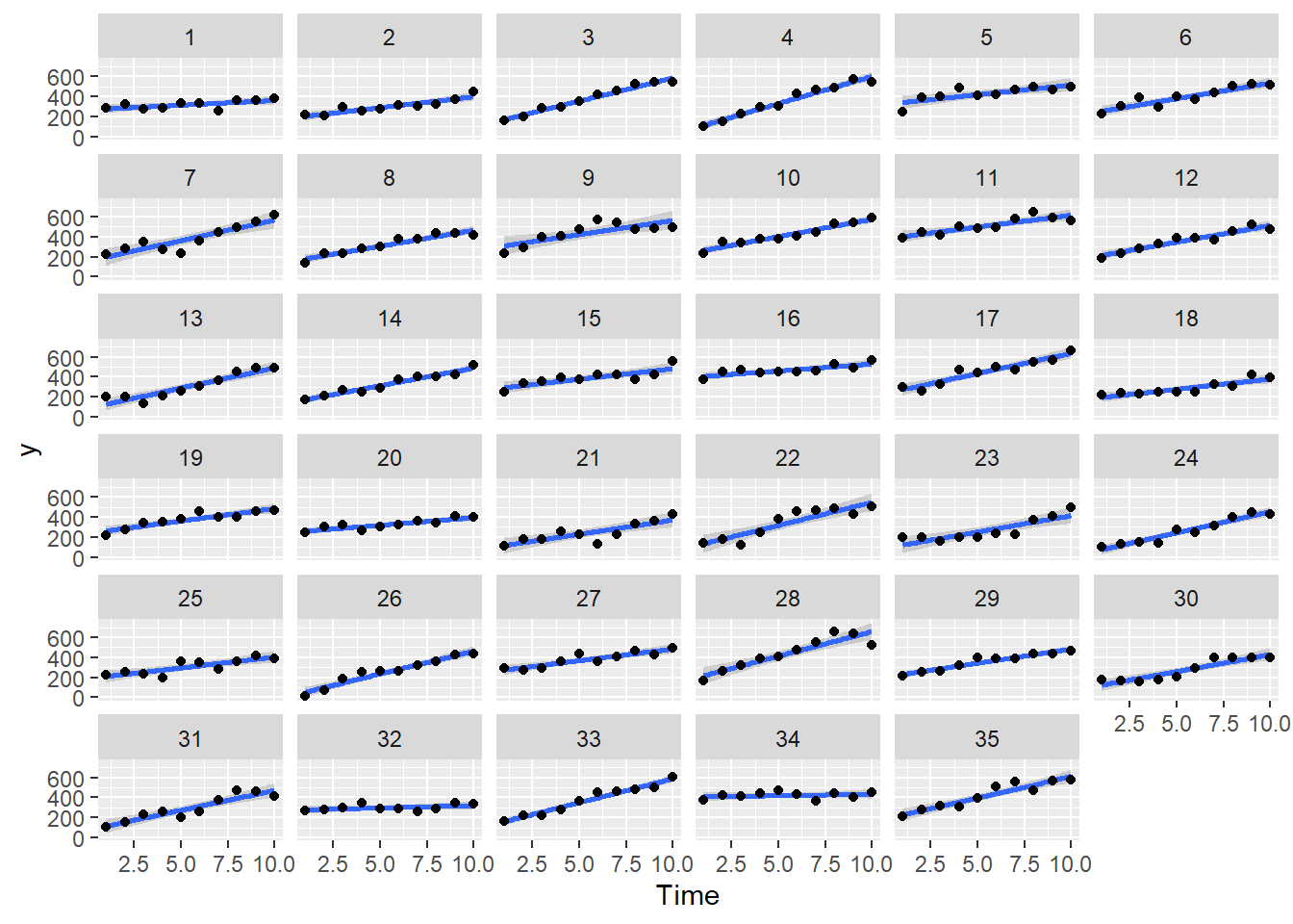

Exploratory data analysis

Normality and Homogeneity of variance

> boxplot(y~Time, data.rm)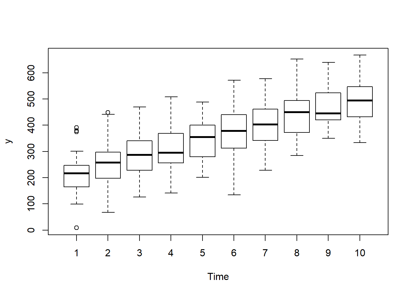

> 
> ggplot(data.rm, aes(y=y, x=factor(Time))) + geom_boxplot()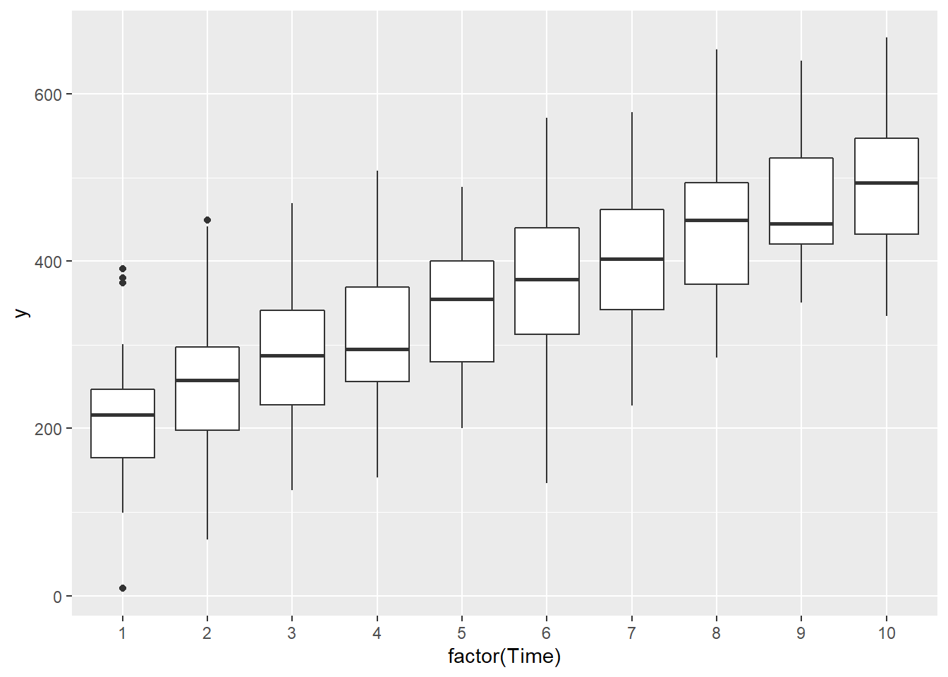

Conclusions:

there is no evidence that the response variable is consistently non-normal across all populations - each boxplot is approximately symmetrical.
there is no evidence that variance (as estimated by the height of the boxplots) differs between the five populations. More importantly, there is no evidence of a relationship between mean and variance - the height of boxplots does not increase with increasing position along the \(y\)-axis. Hence it there is no evidence of non-homogeneity

Obvious violations could be addressed either by:

transform the scale of the response variables (to address normality, etc). Note transformations should be applied to the entire response variable (not just those populations that are skewed).

Block by within-Block interaction

> with(data.rm, interaction.plot(Time,Block,y))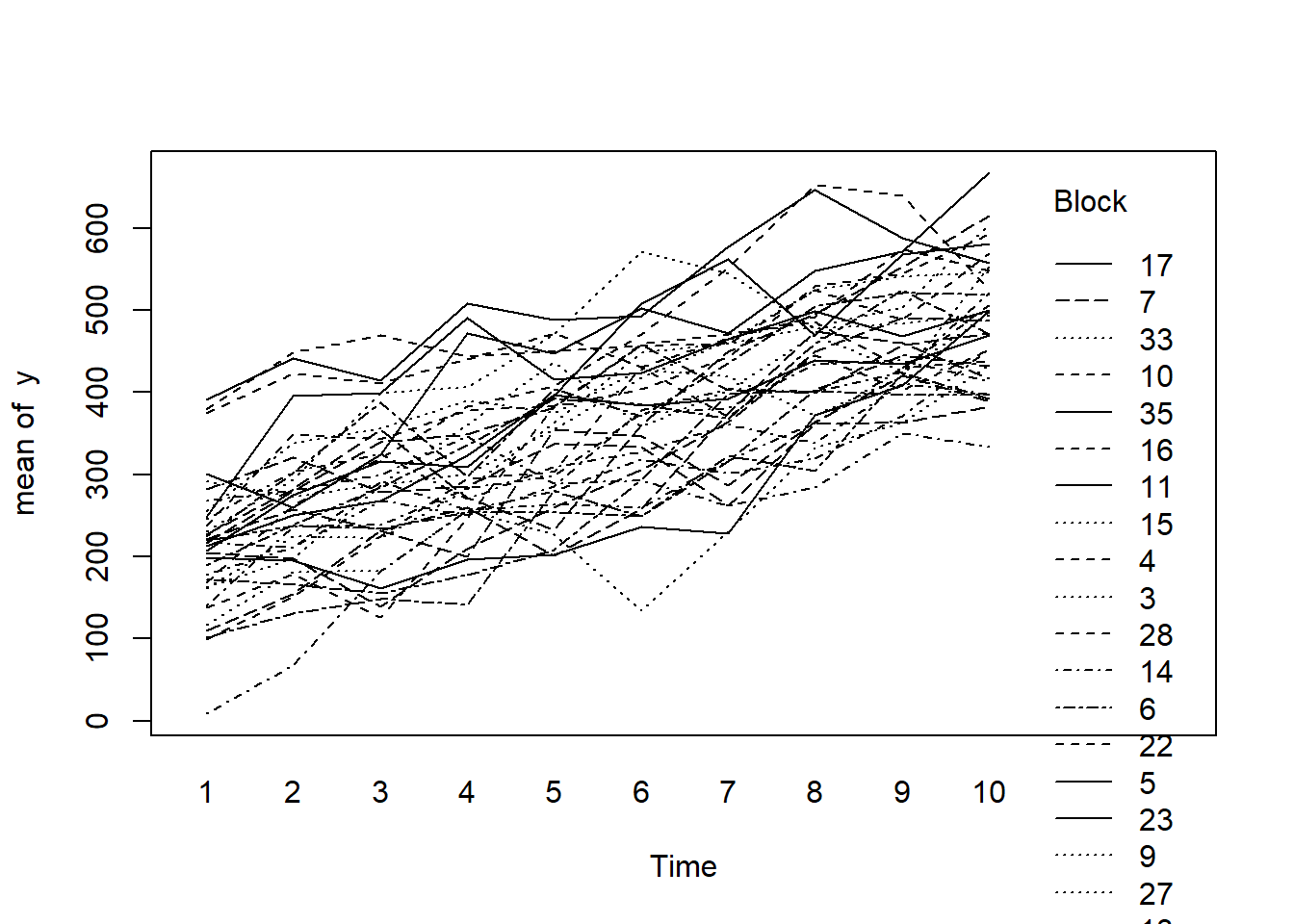

> 
> ggplot(data.rm, aes(y=y, x=Time, color=Block, group=Block)) + geom_line() +
+   guides(color=guide_legend(ncol=3))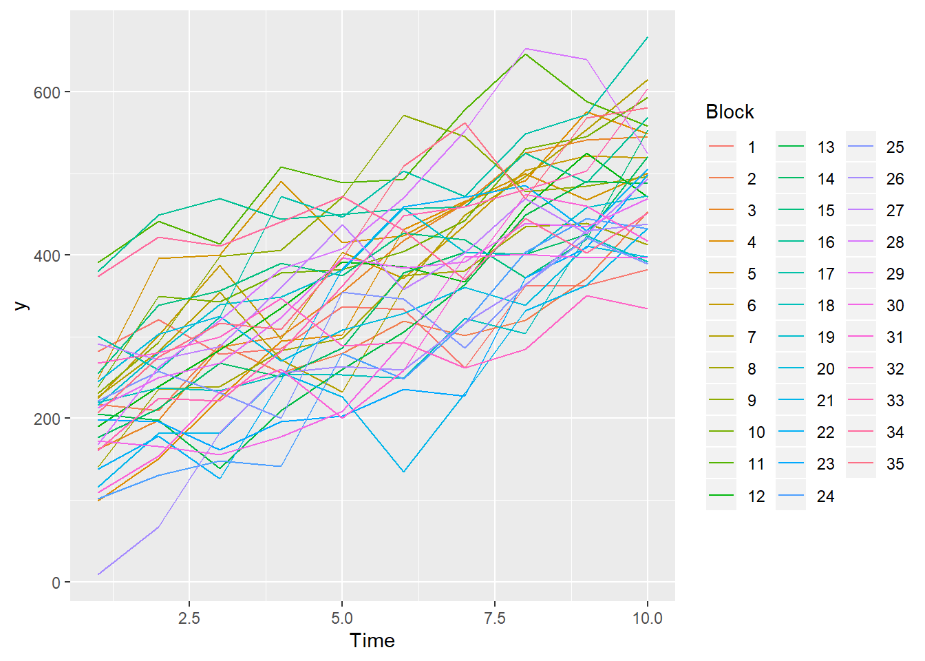

> 
> residualPlots(lm(y~Block+Time, data.rm))

           Test stat Pr(>|Test stat|)
Block                                
Time         -0.7274           0.4675
Tukey test   -0.9809           0.3267
> 
> # the Tukey's non-additivity test by itself can be obtained via an internal function
> # within the car package
> car:::tukeyNonaddTest(lm(y~Block+Time, data.rm))
      Test     Pvalue 
-0.9808606  0.3266615 
> 
> # alternatively, there is also a Tukey's non-additivity test within the
> # asbio package
> with(data.rm,tukey.add.test(y,Time,Block))

Tukey's one df test for additivity 
F = 0.3997341   Denom df = 305    p-value = 0.5277003

Conclusions:

there is no visual or inferential evidence of any major interactions between Block and the within-Block effect (Time). Any trends appear to be reasonably consistent between Blocks.

Sphericity

Since the levels of Time cannot be randomly assigned, it is likely that sphericity is not met. We can explore whether there is an auto-correlation patterns in the residuals. Note, as there was only ten time periods, it does not make logical sense to explore lags above \(10\).

> library(nlme)
> data.rm.lme <- lme(y~Time, random=~1|Block, data=data.rm)
> acf(resid(data.rm.lme), lag=10)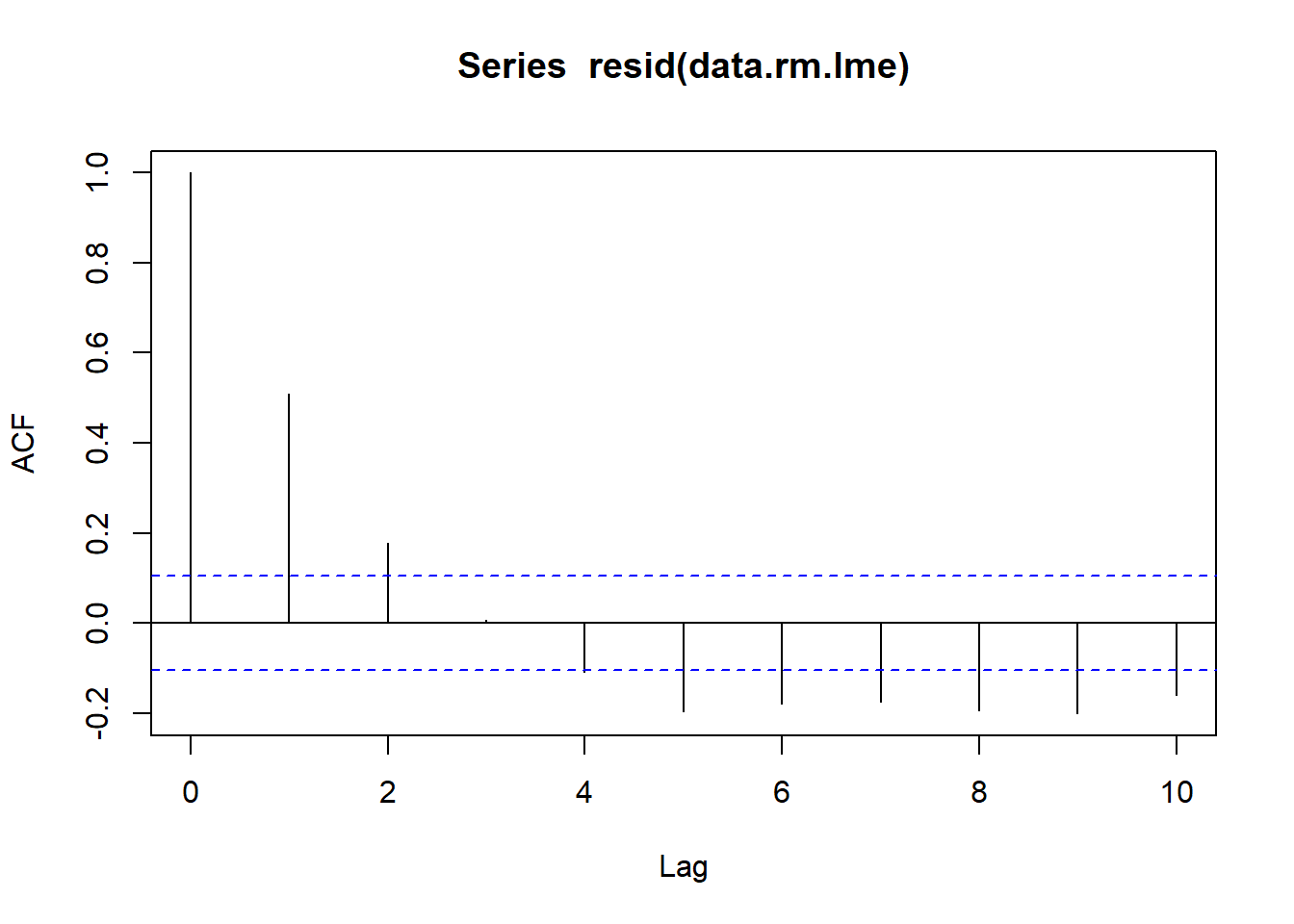

Conclusions:

The autocorrelation factor (ACF) at a range of lags up to \(10\), indicate that there is a cyclical pattern of residual auto-correlation. We really should explore incorporating some form of correlation structure into our model.

Model fitting

Matrix parameterisation

> rstanString2="
+ data{
+    int n;
+    int nX;
+    int nB;
+    vector [n] y;
+    matrix [n,nX] X;
+    int B[n];
+ }
+ 
+ parameters{
+   vector [nX] beta;
+   real<lower=0> sigma;
+   vector [nB] gamma;
+   real<lower=0> sigma_B;
+ }
+ transformed parameters {
+   vector[n] mu;    
+   
+   mu = X*beta;
+   for (i in 1:n) {
+     mu[i] = mu[i] + gamma[B[i]];
+   }
+ } 
+ model{
+     // Priors
+     beta ~ normal( 0 , 100 );
+     gamma ~ normal( 0 , sigma_B );
+     sigma_B ~ cauchy( 0 , 25 );
+     sigma ~ cauchy( 0 , 25 );
+     
+     y ~ normal( mu , sigma );
+ }
+ 
+ "
> 
> ## write the model to a text file
> writeLines(rstanString2, con = "matrixModel2.stan")
> 
> Xmat <- model.matrix(~Time, data=data.rm)
> data.rm.list <- with(data.rm, list(y=y, X=Xmat, nX=ncol(Xmat),
+   B=as.numeric(Block),
+   n=nrow(data.rm), nB=length(levels(Block))))
> 
> params <- c('beta','sigma','sigma_B')
> burnInSteps = 3000
> nChains = 2
> numSavedSteps = 3000
> thinSteps = 1
> nIter = burnInSteps+ceiling((numSavedSteps * thinSteps)/nChains)
> 
> data.rm.rstan.d  <- stan(data = data.rm.list, file = "matrixModel2.stan", 
+                             chains = nChains, pars = params, iter = nIter, 
+                             warmup = burnInSteps, thin = thinSteps)

SAMPLING FOR MODEL 'matrixModel' NOW (CHAIN 1).
Chain 1: 
Chain 1: Gradient evaluation took 0 seconds
Chain 1: 1000 transitions using 10 leapfrog steps per transition would take 0 seconds.
Chain 1: Adjust your expectations accordingly!
Chain 1: 
Chain 1: 
Chain 1: Iteration:    1 / 4500 [  0%]  (Warmup)
Chain 1: Iteration:  450 / 4500 [ 10%]  (Warmup)
Chain 1: Iteration:  900 / 4500 [ 20%]  (Warmup)
Chain 1: Iteration: 1350 / 4500 [ 30%]  (Warmup)
Chain 1: Iteration: 1800 / 4500 [ 40%]  (Warmup)
Chain 1: Iteration: 2250 / 4500 [ 50%]  (Warmup)
Chain 1: Iteration: 2700 / 4500 [ 60%]  (Warmup)
Chain 1: Iteration: 3001 / 4500 [ 66%]  (Sampling)
Chain 1: Iteration: 3450 / 4500 [ 76%]  (Sampling)
Chain 1: Iteration: 3900 / 4500 [ 86%]  (Sampling)
Chain 1: Iteration: 4350 / 4500 [ 96%]  (Sampling)
Chain 1: Iteration: 4500 / 4500 [100%]  (Sampling)
Chain 1: 
Chain 1:  Elapsed Time: 2.027 seconds (Warm-up)
Chain 1:                0.657 seconds (Sampling)
Chain 1:                2.684 seconds (Total)
Chain 1: 

SAMPLING FOR MODEL 'matrixModel' NOW (CHAIN 2).
Chain 2: 
Chain 2: Gradient evaluation took 0 seconds
Chain 2: 1000 transitions using 10 leapfrog steps per transition would take 0 seconds.
Chain 2: Adjust your expectations accordingly!
Chain 2: 
Chain 2: 
Chain 2: Iteration:    1 / 4500 [  0%]  (Warmup)
Chain 2: Iteration:  450 / 4500 [ 10%]  (Warmup)
Chain 2: Iteration:  900 / 4500 [ 20%]  (Warmup)
Chain 2: Iteration: 1350 / 4500 [ 30%]  (Warmup)
Chain 2: Iteration: 1800 / 4500 [ 40%]  (Warmup)
Chain 2: Iteration: 2250 / 4500 [ 50%]  (Warmup)
Chain 2: Iteration: 2700 / 4500 [ 60%]  (Warmup)
Chain 2: Iteration: 3001 / 4500 [ 66%]  (Sampling)
Chain 2: Iteration: 3450 / 4500 [ 76%]  (Sampling)
Chain 2: Iteration: 3900 / 4500 [ 86%]  (Sampling)
Chain 2: Iteration: 4350 / 4500 [ 96%]  (Sampling)
Chain 2: Iteration: 4500 / 4500 [100%]  (Sampling)
Chain 2: 
Chain 2:  Elapsed Time: 2.764 seconds (Warm-up)
Chain 2:                0.453 seconds (Sampling)
Chain 2:                3.217 seconds (Total)
Chain 2: 
> 
> print(data.rm.rstan.d , par = c('beta','sigma','sigma_B'))
Inference for Stan model: matrixModel.
2 chains, each with iter=4500; warmup=3000; thin=1; 
post-warmup draws per chain=1500, total post-warmup draws=3000.

          mean se_mean    sd   2.5%    25%    50%    75%  97.5% n_eff Rhat
beta[1] 185.90    0.79 12.77 159.70 177.57 185.87 194.16 211.22   263 1.01
beta[2]  30.80    0.02  1.03  28.72  30.13  30.77  31.46  32.80  2854 1.00
sigma    55.86    0.04  2.20  51.68  54.34  55.75  57.29  60.43  2639 1.00
sigma_B  64.74    0.21  8.97  50.08  58.37  63.92  70.18  84.68  1816 1.00

Samples were drawn using NUTS(diag_e) at Thu Feb 20 11:15:03 2020.
For each parameter, n_eff is a crude measure of effective sample size,
and Rhat is the potential scale reduction factor on split chains (at 
convergence, Rhat=1).

Given that Time cannot be randomized, there is likely to be a temporal dependency structure to the data. The above analyses assume no temporal dependency - actually, they assume that the variance-covariance matrix demonstrates a structure known as sphericity. Lets specifically model in a first order autoregressive correlation structure in an attempt to accommodate the expected temporal autocorrelation.

> rstanString3="
+ data{
+    int n;
+    int nX;
+    int nB;
+    vector [n] y;
+    matrix [n,nX] X;
+    int B[n];
+    vector [n] tgroup;
+ }
+ 
+ parameters{
+   vector [nX] beta;
+   real<lower=0> sigma;
+   vector [nB] gamma;
+   real<lower=0> sigma_B;
+   real ar;
+ }
+ transformed parameters {
+   vector[n] mu;    
+   vector[n] E;
+   vector[n] res;
+ 
+   mu = X*beta;
+   for (i in 1:n) {
+      E[i] = 0;
+   }
+   for (i in 1:n) {
+     mu[i] = mu[i] + gamma[B[i]];
+     res[i] = y[i] - mu[i];
+   if(i>0 && i < n && tgroup[i+1] == tgroup[i]) {
+     E[i+1] = res[i];
+     }
+     mu[i] = mu[i] + (E[i] * ar);
+   }
+ } 
+ model{
+     // Priors
+     beta ~ normal( 0 , 100 );
+     gamma ~ normal( 0 , sigma_B );
+     sigma_B ~ cauchy( 0 , 25 );
+     sigma ~ cauchy( 0 , 25 );
+     
+     y ~ normal( mu , sigma );
+ }
+ 
+ "
> 
> ## write the model to a text file
> writeLines(rstanString3, con = "matrixModel3.stan")
> 
> Xmat <- model.matrix(~Time, data=data.rm)
> data.rm.list <- with(data.rm, list(y=y, X=Xmat, nX=ncol(Xmat),
+   B=as.numeric(Block),
+   n=nrow(data.rm), nB=length(levels(Block)),
+   tgroup=as.numeric(Block)))
> 
> params <- c('beta','sigma','sigma_B','ar')
> burnInSteps = 3000
> nChains = 2
> numSavedSteps = 3000
> thinSteps = 1
> nIter = burnInSteps+ceiling((numSavedSteps * thinSteps)/nChains)
> 
> data.rm.rstan.d  <- stan(data = data.rm.list, file = "matrixModel3.stan", 
+                             chains = nChains, pars = params, iter = nIter, 
+                             warmup = burnInSteps, thin = thinSteps)

SAMPLING FOR MODEL 'matrixModel3' NOW (CHAIN 1).
Chain 1: 
Chain 1: Gradient evaluation took 0 seconds
Chain 1: 1000 transitions using 10 leapfrog steps per transition would take 0 seconds.
Chain 1: Adjust your expectations accordingly!
Chain 1: 
Chain 1: 
Chain 1: Iteration:    1 / 4500 [  0%]  (Warmup)
Chain 1: Iteration:  450 / 4500 [ 10%]  (Warmup)
Chain 1: Iteration:  900 / 4500 [ 20%]  (Warmup)
Chain 1: Iteration: 1350 / 4500 [ 30%]  (Warmup)
Chain 1: Iteration: 1800 / 4500 [ 40%]  (Warmup)
Chain 1: Iteration: 2250 / 4500 [ 50%]  (Warmup)
Chain 1: Iteration: 2700 / 4500 [ 60%]  (Warmup)
Chain 1: Iteration: 3001 / 4500 [ 66%]  (Sampling)
Chain 1: Iteration: 3450 / 4500 [ 76%]  (Sampling)
Chain 1: Iteration: 3900 / 4500 [ 86%]  (Sampling)
Chain 1: Iteration: 4350 / 4500 [ 96%]  (Sampling)
Chain 1: Iteration: 4500 / 4500 [100%]  (Sampling)
Chain 1: 
Chain 1:  Elapsed Time: 4.063 seconds (Warm-up)
Chain 1:                1.041 seconds (Sampling)
Chain 1:                5.104 seconds (Total)
Chain 1: 

SAMPLING FOR MODEL 'matrixModel3' NOW (CHAIN 2).
Chain 2: 
Chain 2: Gradient evaluation took 0 seconds
Chain 2: 1000 transitions using 10 leapfrog steps per transition would take 0 seconds.
Chain 2: Adjust your expectations accordingly!
Chain 2: 
Chain 2: 
Chain 2: Iteration:    1 / 4500 [  0%]  (Warmup)
Chain 2: Iteration:  450 / 4500 [ 10%]  (Warmup)
Chain 2: Iteration:  900 / 4500 [ 20%]  (Warmup)
Chain 2: Iteration: 1350 / 4500 [ 30%]  (Warmup)
Chain 2: Iteration: 1800 / 4500 [ 40%]  (Warmup)
Chain 2: Iteration: 2250 / 4500 [ 50%]  (Warmup)
Chain 2: Iteration: 2700 / 4500 [ 60%]  (Warmup)
Chain 2: Iteration: 3001 / 4500 [ 66%]  (Sampling)
Chain 2: Iteration: 3450 / 4500 [ 76%]  (Sampling)
Chain 2: Iteration: 3900 / 4500 [ 86%]  (Sampling)
Chain 2: Iteration: 4350 / 4500 [ 96%]  (Sampling)
Chain 2: Iteration: 4500 / 4500 [100%]  (Sampling)
Chain 2: 
Chain 2:  Elapsed Time: 3.945 seconds (Warm-up)
Chain 2:                1.015 seconds (Sampling)
Chain 2:                4.96 seconds (Total)
Chain 2: 
> 
> print(data.rm.rstan.d , par = c('beta','sigma','sigma_B','ar'))
Inference for Stan model: matrixModel3.
2 chains, each with iter=4500; warmup=3000; thin=1; 
post-warmup draws per chain=1500, total post-warmup draws=3000.

          mean se_mean    sd   2.5%    25%    50%    75%  97.5% n_eff Rhat
beta[1] 179.26    0.24 12.87 153.98 170.50 179.54 187.94 203.70  2981    1
beta[2]  31.25    0.02  1.64  28.05  30.14  31.22  32.32  34.54  5531    1
sigma    48.74    0.03  1.96  45.11  47.43  48.64  50.04  52.87  3537    1
sigma_B  50.33    0.30 10.54  31.10  43.06  49.68  56.96  72.38  1241    1
ar        0.78    0.00  0.05   0.68   0.75   0.78   0.82   0.87  2773    1

Samples were drawn using NUTS(diag_e) at Thu Feb 20 11:15:58 2020.
For each parameter, n_eff is a crude measure of effective sample size,
and Rhat is the potential scale reduction factor on split chains (at 
convergence, Rhat=1).

References

Gelman, Andrew, Daniel Lee, and Jiqiang Guo. 2015. “Stan: A Probabilistic Programming Language for Bayesian Inference and Optimization.” Journal of Educational and Behavioral Statistics 40 (5): 530–43.

Stan Development Team. 2018. “RStan: The R Interface to Stan.” http://mc-stan.org/.

tutorials STAN randomised complete block anova

Randomised Complete Block Anova - STAN

Overview

Introduction

Linear models

Assumptions

Simple RCB

Data generation

Exploratory data analysis

Model fitting

Full means parameterisation

Full effect parameterisation

Matrix parameterisation

RCB (repeated measures) - continuous within

Data generation

Exploratory data analysis

Model fitting

Matrix parameterisation

References

Related