Temporal Autocorrelation (JAGS)

Last updated on Feb 8, 2020 autocorrelation, JAGS, R

This tutorial will focus on the use of Bayesian estimation to fit simple linear regression models. BUGS (Bayesian inference Using Gibbs Sampling) is an algorithm and supporting language (resembling R) dedicated to performing the Gibbs sampling implementation of Markov Chain Monte Carlo (MCMC) method. Dialects of the BUGS language are implemented within three main projects:

OpenBUGS - written in component pascal.
JAGS - (Just Another Gibbs Sampler) - written in C++.
STAN - a dedicated Bayesian modelling framework written in C++ and implementing Hamiltonian MCMC samplers.

Whilst the above programs can be used stand-alone, they do offer the rich data pre-processing and graphical capabilities of R, and thus, they are best accessed from within R itself. As such there are multiple packages devoted to interfacing with the various software implementations:

R2OpenBUGS - interfaces with OpenBUGS
R2jags - interfaces with JAGS
rstan - interfaces with STAN

This tutorial will demonstrate how to fit models in JAGS (Plummer (2004)) using the package R2jags (Su et al. (2015)) as interface, which also requires to load some other packages.

Overview

Introduction

Up until now (in the proceeding tutorials), the focus has been on models that adhere to specific assumptions about the underlying populations (and data). Indeed, both before and immediately after fitting these models, I have stressed the importance of evaluating and validating the proposed and fitted models to ensure reliability of the models. It is now worth us revisiting those fundamental assumptions as well as exploring the options that are available when the populations (data) do not conform. Let’s explore a simple linear regression model to see how each of the assumptions relate to the model.

\[ y_i = \beta_0 + \beta_1x_i + \epsilon_i \;\;\; \text{with} \;\;\; \epsilon_i \sim \text{Normal}(0, \sigma^2).\]

The above simple statistical model models the linear relationship of \(y_i\) against \(x_i\). The residuals (\(\epsilon\)) are assumed to be normally distributed with a mean of zero and a constant (yet unknown) variance (\(\sigma\), homogeneity of variance). The residuals (and thus observations) are also assumed to all be independent.

Homogeneity of variance and independence are encapsulated within the single symbol for variance (\(\sigma^2\)). In assuming equal variances and independence, we are actually making an assumption about the variance-covariance structure of the populations (and thus residuals). Specifically, we assume that all populations are equally varied and thus can be represented well by a single variance term (all diagonal values in a \(N\times N\) covariance matrix are the same, \(\sigma^2\)) and the covariances between each population are zero (off diagonals). In simple regression, each observation (data point) represents a single observation drawn (sampled) from an entire population of possible observations. The above covariance structure thus assumes that the covariance between each population (observation) is zero - that is, each observation is completely independent of each other observation. Whilst it is mathematically convenient when data conform to these conditions (normality, homogeneity of variance, independence and linearity), data often violate one or more of these assumptions. In the following, I want to discuss and explore the causes and options for dealing with non-compliance to each of these conditions. By gaining a better understanding of how the various model fitting engines perform their task, we are better equipped to accommodate aspects of the data that don’t otherwise conform to the simple regression assumptions. In this tutorial we specifically focus on the topic of heterogeneity of the variance.

In order that the estimated parameters represent the underlying populations in an unbiased manner, the residuals (and thus each each observation) must be independent. However, what if we were sampling a population over time and we were interested in investigating how changes in a response relate to changes in a predictor (such as rainfall). For any response that does not “reset” itself on a regular basis, the state of the population (the value of its response) at a given time is likely to be at least partly dependent on the state of the population at the sampling time before. We can further generalise the above into:

\[ y_i \sim Dist(\mu_i),\]

where \(\mu_i=\boldsymbol X \boldsymbol \beta + \boldsymbol Z \boldsymbol \gamma\), with \(\boldsymbol X\) and \(\boldsymbol \beta\) representing the fixed data structure and fixed effects, respectively, while with \(\boldsymbol Z\) and \(\boldsymbol \gamma\) represent the varying data structure and varying effects, respectively. In simple regression, there are no “varying” effects, and thus:

\[ \boldsymbol \gamma \sim MVN(\boldsymbol 0, \boldsymbol \Sigma),\]

where \(\boldsymbol \Sigma\) is a variance-covariance matrix of the form

\[ \boldsymbol \Sigma = \frac{\sigma^2}{1-\rho^2} \begin{bmatrix} 1 & \rho^{\phi_{1,2}} & \ldots & \rho^{\phi_{1,n}} \\ \rho^{\phi_{2,1}} & 1 & \ldots & \vdots\\ \vdots & \ldots & 1 & \vdots\\ \rho^{\phi_{n,1}} & \ldots & \ldots & 1 \end{bmatrix}. \]

Notice that this introduces a very large number of additional parameters that require estimating: \(\sigma^2\) (error variance), \(\rho\) (base autocorrelation) and each of the individual covariances (\(\rho^{\phi_{n,n}}\)). Hence, there are always going to be more parameters to estimate than there are date avaiable to use to estimate these paramters. We typically make one of a number of alternative assumptions so as to make this task more manageable.

When we assume that all residuals are independent (regular regression), i.e. \(\rho=0\), \(\boldsymbol \Sigma\) is essentially equal to \(\sigma^2 \boldsymbol I\) and we simply use:

\[ \boldsymbol \gamma \sim N( 0,\sigma^2).\]

We could assume there is a reasonably simple pattern of correlation that declines over time. The simplest of these is a first order autoregressive (AR1) structure in which exponent on the correlation declines linearly according to the time lag (\(\mid t - s\mid\)).

\[ \boldsymbol \Sigma = \frac{\sigma^2}{1-\rho^2} \begin{bmatrix} 1 & \rho & \ldots & \rho^{\mid t-s \mid} \\ \rho & 1 & \ldots & \vdots\\ \vdots & \ldots & 1 & \vdots\\ \rho^{\mid t-s \mid } & \ldots & \ldots & 1 \end{bmatrix}. \]

Note, in making this assumption, we are also assuming that the degree of correlation is dependent only on the lag and not on when the lag occurs (stationarity). That is all lag 1 residual pairs will have the same degree of correlation, all the lag \(2\) pairs will have the same correlation and so on.

First order autocorrelation

Consider an example, in which the number of individuals at time \(2\) will be partly dependent on the number of individuals present at time \(1\). Clearly then, the observations (and thus residuals) are not fully independent - there is an auto-regressive correlation dependency structure. We could accommodate this lack of independence by fitting a model that incorporates a AR1 variance-covariance structure. Alternatively, we fit the following model:

\[ y_{it} \sim Dist(\mu_{it}),\]

where

\[\mu_{it}=\boldsymbol X \boldsymbol \beta + \rho \epsilon_{i,t-1} + \gamma_{it},\]

and where \(\gamma \sim N(0, \sigma^2)\). In this version of the model, we are stating that the expected value of an observation is equal to the regular linear predictor plus the autocorrelation parameter (\(\rho\)) multipled by the residual associated with the previous observation plus the regular independently distributed noise (\(\sigma^2\)). Such a model is substantially faster to fit, although along with stationarity assumes in estimating the autocorrelation parameter, only the smallest lags are used. To see this in action, we will first generate some temporally auto-correlated data.

> set.seed(126)
> n = 50
> a <- 20  #intercept
> b <- 0.2  #slope
> x <- round(runif(n, 1, n), 1)  #values of the year covariate
> year <- 1:n
> sigma <- 20
> rho <- 0.8
> 
> library(nlme)
> ## define a constructor for a first-order
> ## correlation structure
> ar1 <- corAR1(form = ~year, value = rho)
> ## initialize this constructor against our data
> AR1 <- Initialize(ar1, data = data.frame(year))
> ## generate a correlation matrix
> V <- corMatrix(AR1)
> ## Cholesky factorization of V
> Cv <- chol(V)
> ## simulate AR1 errors
> e <- t(Cv) %*% rnorm(n, 0, sigma)  # cov(e) = V * sig^2
> ## generate response
> y <- a + b * x + e
> data.temporalCor = data.frame(y = y, x = x, year = year)
> write.table(data.temporalCor, file = "data.temporalCor.csv",
+     sep = ",", quote = F, row.names = FALSE)
> 
> pairs(data.temporalCor)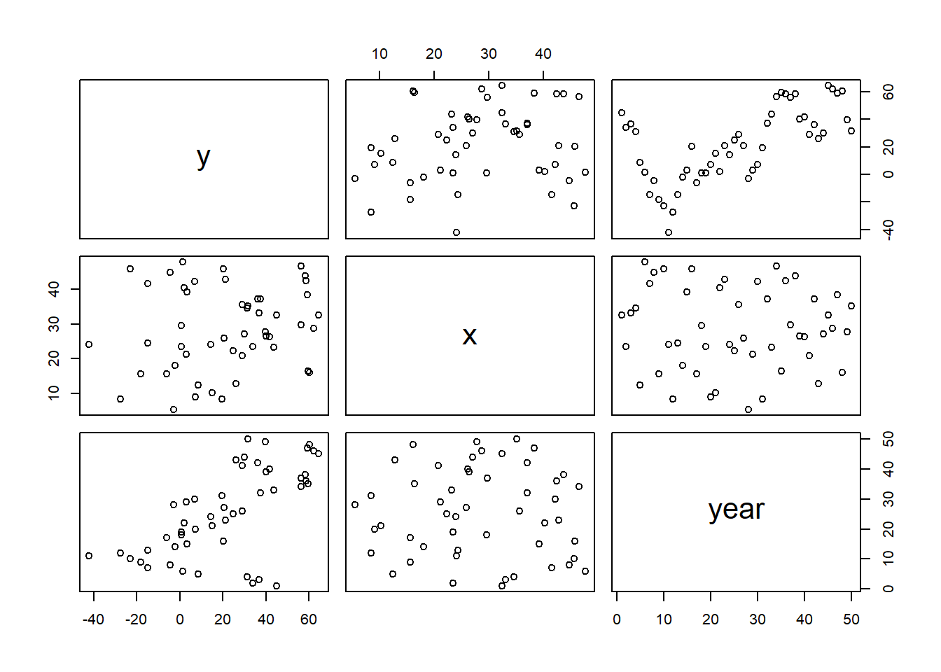

We will now proceed to analyse these data via both of the above techniques for JAGS:

incorporating AR1 residual autocorrelation structure
incorporating lagged residuals into the model

Incorporating lagged residuals

Model fitting

We proceed to code the model into JAGS (remember that in this software normal distribution are parameterised in terms of precisions \(\tau\) rather than variances, where \(\tau=\frac{1}{\sigma^2}\)). Define the model.

> modelString = " 
+   model {
+   #Likelihood
+   for (i in 1:n) {
+   fit[i] <- inprod(beta[],X[i,])
+   y[i] ~ dnorm(mu[i],tau.cor)
+   }
+   e[1] <- (y[1] - fit[1])
+   mu[1] <- fit[1]
+   for (i in 2:n) {
+   e[i] <- (y[i] - fit[i]) #- phi*e[i-1]
+   mu[i] <- fit[i] + phi * e[i-1]
+   }
+   #Priors
+   phi ~ dunif(-1,1)
+   for (i in 1:nX) {
+   beta[i] ~ dnorm(0,1.0E-6)
+   }
+   sigma <- z/sqrt(chSq)    # prior for sigma; cauchy = normal/sqrt(chi^2)
+   z ~ dnorm(0, 0.04)I(0,)
+   chSq ~ dgamma(0.5, 0.5)  # chi^2 with 1 d.f.
+   tau <- pow(sigma, -2)
+   tau.cor <- tau #* (1- phi*phi)
+   }
+   "
> 
> ## write the model to a text file
> writeLines(modelString, con = "tempModel.txt")

Arrange the data as a list (as required by JAGS). As input, JAGS will need to be supplied with: the response variable, the predictor matrix, the number of predictors, the total number of observed items. This all needs to be contained within a list object. We will create two data lists, one for each of the hypotheses.

> Xmat = model.matrix(~x, data.temporalCor)
> data.temporalCor.list <- with(data.temporalCor, list(y = y, X = Xmat,
+     n = nrow(data.temporalCor), nX = ncol(Xmat)))

Define the nodes (parameters and derivatives) to monitor and the chain parameters.

> params <- c("beta", "sigma", "phi")
> nChains = 2
> burnInSteps = 5000
> thinSteps = 1
> numSavedSteps = 10000  #across all chains
> nIter = ceiling(burnInSteps + (numSavedSteps * thinSteps)/nChains)
> nIter
[1] 10000

Start the JAGS model (check the model, load data into the model, specify the number of chains and compile the model). Load the R2jags package.

> library(R2jags)

Now run the JAGS code via the R2jags interface.

> data.temporalCor.r2jags <- jags(data = data.temporalCor.list, inits = NULL, parameters.to.save = params,
+     model.file = "tempModel.txt", n.chains = nChains, n.iter = nIter,
+     n.burnin = burnInSteps, n.thin = thinSteps)
Compiling model graph
   Resolving undeclared variables
   Allocating nodes
Graph information:
   Observed stochastic nodes: 50
   Unobserved stochastic nodes: 5
   Total graph size: 413

Initializing model
> 
> print(data.temporalCor.r2jags)
Inference for Bugs model at "tempModel.txt", fit using jags,
 2 chains, each with 10000 iterations (first 5000 discarded)
 n.sims = 10000 iterations saved
         mu.vect sd.vect    2.5%     25%     50%     75%   97.5%  Rhat n.eff
beta[1]   30.841  11.858   8.852  22.556  30.505  38.559  55.177 1.001 10000
beta[2]    0.225   0.100   0.028   0.159   0.225   0.292   0.422 1.001  3800
phi        0.913   0.054   0.793   0.879   0.919   0.954   0.994 1.001  3400
sigma     12.133   1.253   9.967  11.253  12.034  12.902  14.828 1.001  7300
deviance 391.602   2.641 388.354 389.656 390.985 392.927 398.180 1.001  9200

For each parameter, n.eff is a crude measure of effective sample size,
and Rhat is the potential scale reduction factor (at convergence, Rhat=1).

DIC info (using the rule, pD = var(deviance)/2)
pD = 3.5 and DIC = 395.1
DIC is an estimate of expected predictive error (lower deviance is better).

MCMC diagnostics

> library(mcmcplots)
> denplot(data.temporalCor.r2jags, parms = c("beta", "sigma", "phi"))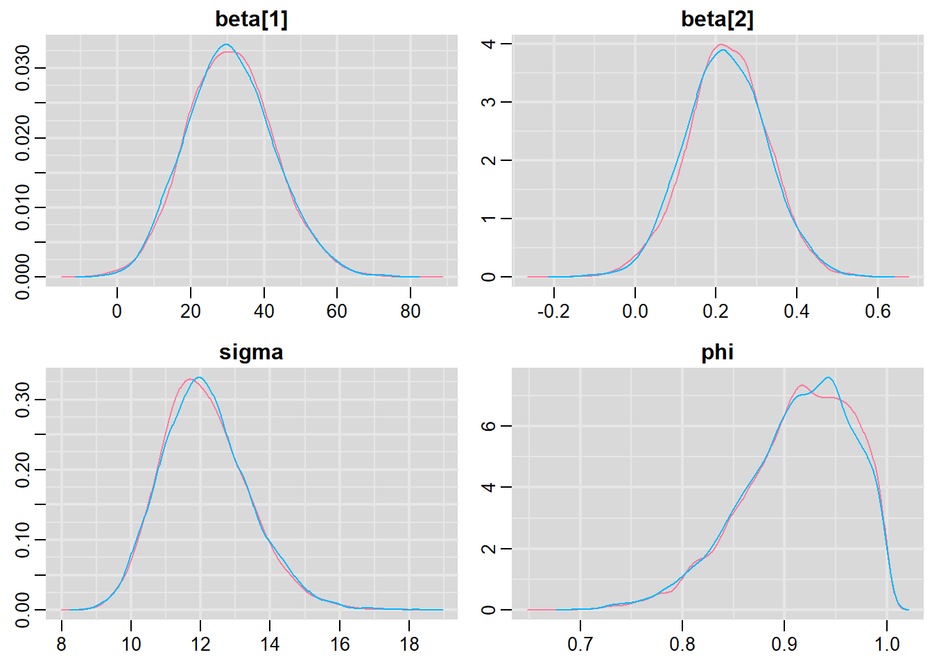

> traplot(data.temporalCor.r2jags, parms = c("beta", "sigma", "phi"))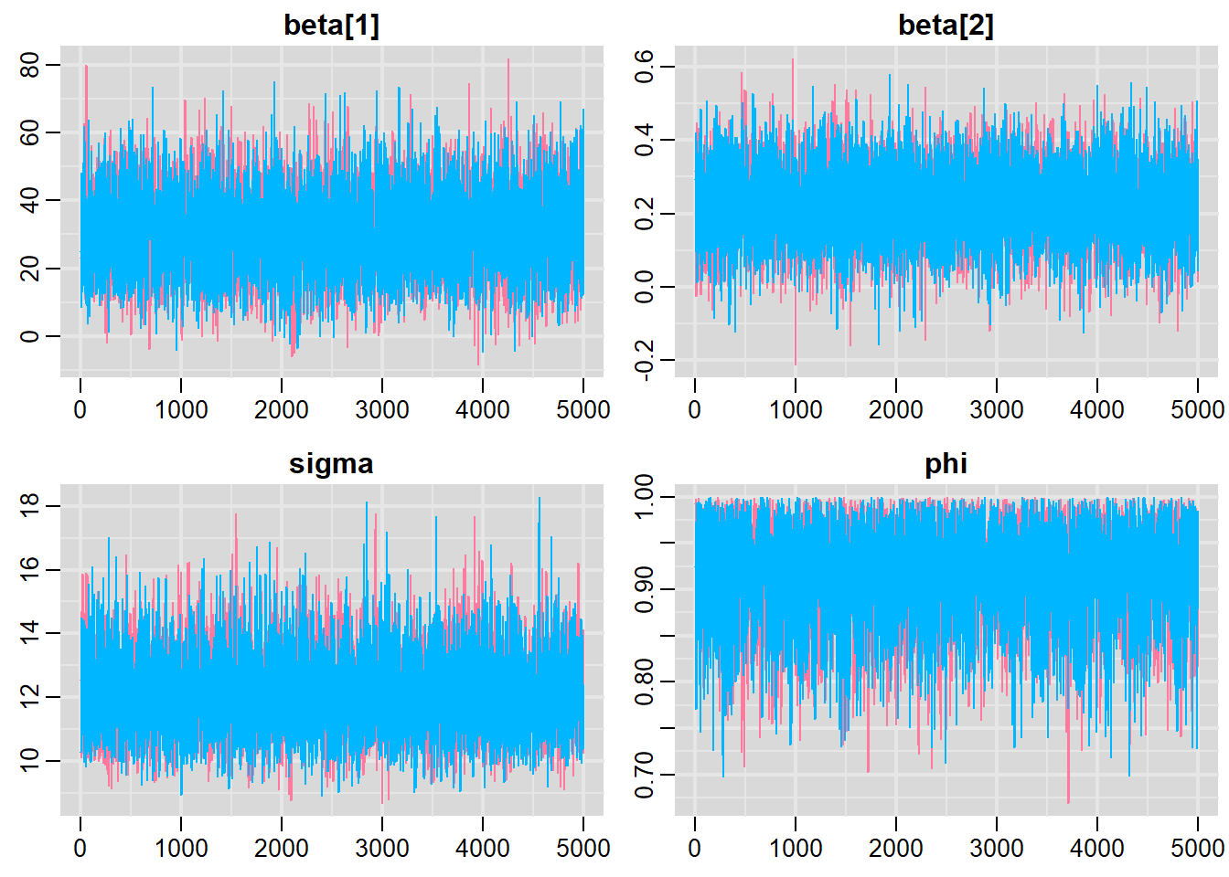

> data.mcmc = as.mcmc(data.temporalCor.r2jags)
> #Raftery diagnostic
> raftery.diag(data.mcmc)
[[1]]

Quantile (q) = 0.025
Accuracy (r) = +/- 0.005
Probability (s) = 0.95 
                                                
          Burn-in  Total Lower bound  Dependence
          (M)      (N)   (Nmin)       factor (I)
 beta[1]  2        3930  3746         1.05      
 beta[2]  2        3866  3746         1.03      
 deviance 2        3866  3746         1.03      
 phi      7        7397  3746         1.97      
 sigma    4        4636  3746         1.24      


[[2]]

Quantile (q) = 0.025
Accuracy (r) = +/- 0.005
Probability (s) = 0.95 
                                                
          Burn-in  Total Lower bound  Dependence
          (M)      (N)   (Nmin)       factor (I)
 beta[1]  3        4062  3746         1.080     
 beta[2]  2        3620  3746         0.966     
 deviance 2        3803  3746         1.020     
 phi      6        6878  3746         1.840     
 sigma    4        4713  3746         1.260

> #Autocorrelation diagnostic
> autocorr.diag(data.mcmc)
           beta[1]      beta[2]     deviance          phi        sigma
Lag 0  1.000000000  1.000000000  1.000000000  1.000000000  1.000000000
Lag 1  0.174857318 -0.006205038  0.164212015  0.398270011  0.166634323
Lag 5  0.017823932  0.002140092 -0.016470982  0.017851360  0.011892997
Lag 10 0.004107514  0.010910488  0.020001216 -0.005693854  0.007020861
Lag 50 0.002176470  0.016102607  0.008360988  0.002061169 -0.007663541

All diagnostics seem fine.

Model validation

Whenever we fit a model that incorporates changes to the variance-covariance structures, we need to explore modified standardized residuals. In this case, the raw residuals should be updated to reflect the autocorrelation (subtract residual from previous time weighted by the autocorrelation parameter) before standardising by sigma.

\[ Res_i = Y_i - \mu_i\]

\[ Res_{i+1} = Res_{i+1} - \rho Res_i\]

\[ Res_i = \frac{Res_i}{\sigma} \]

> mcmc = data.temporalCor.r2jags$BUGSoutput$sims.matrix
> # generate a model matrix
> newdata = data.temporalCor
> Xmat = model.matrix(~x, newdata)
> ## get median parameter estimates
> wch = grep("beta", colnames(mcmc))
> coefs = mcmc[, wch]
> fit = coefs %*% t(Xmat)
> resid = -1 * sweep(fit, 2, data.temporalCor$y, "-")
> n = ncol(resid)
> resid[, -1] = resid[, -1] - (resid[, -n] * mcmc[, "phi"])
> resid = apply(resid, 2, median)/median(mcmc[, "sigma"])
> fit = apply(fit, 2, median)
> 
> library(ggplot2)
> ggplot() + geom_point(data = NULL, aes(y = resid, x = fit)) + theme_classic()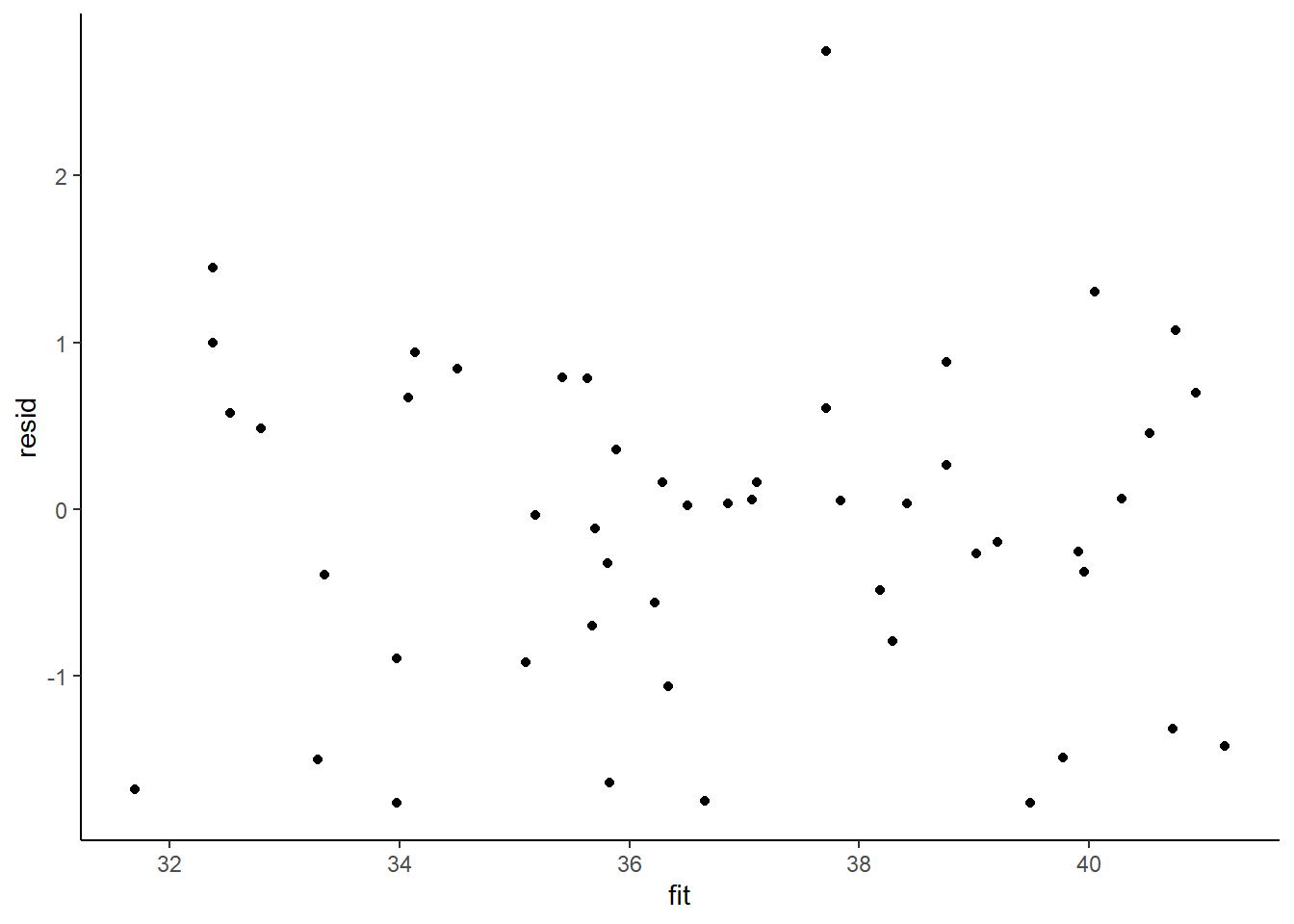

> 
> ggplot() + geom_point(data = NULL, aes(y = resid, x = data.temporalCor$x)) + theme_classic()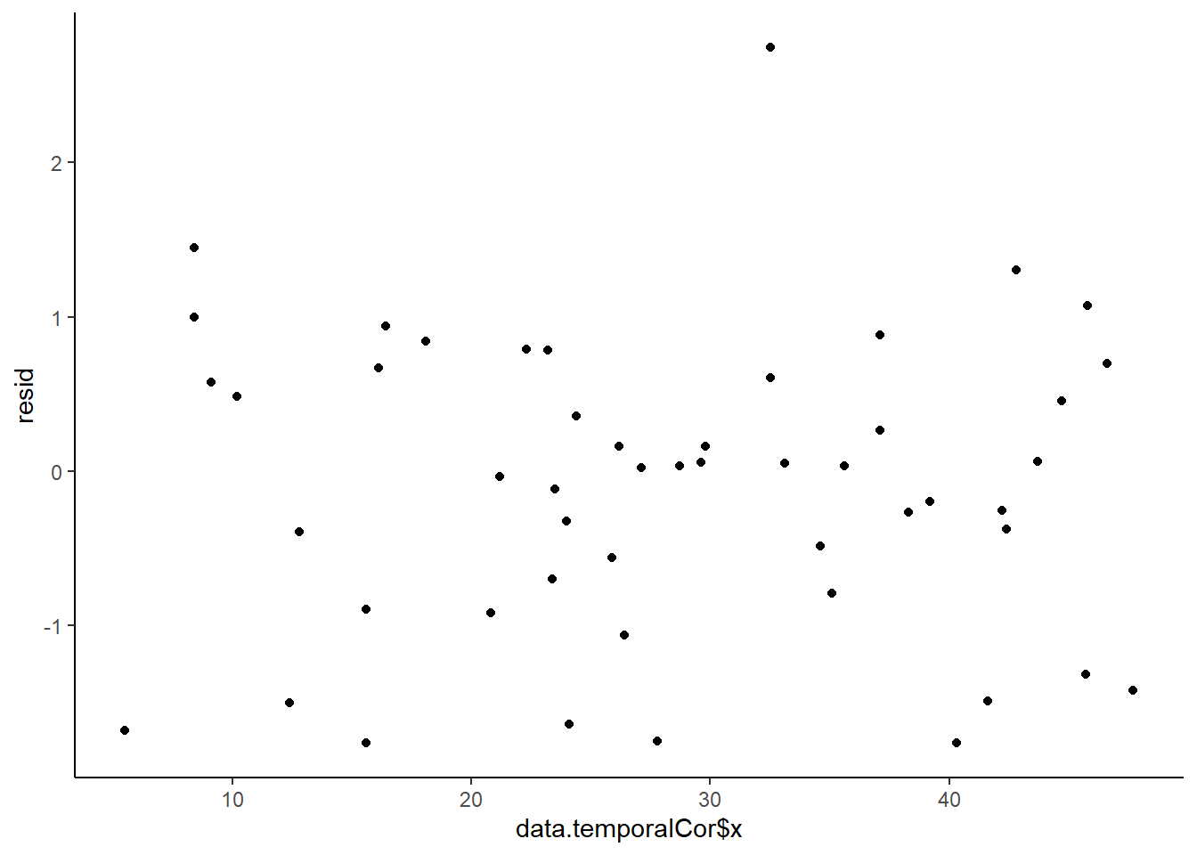

> 
> ggplot(data = NULL, aes(y = resid, x = data.temporalCor$year)) +
+     geom_point() + geom_line() + geom_hline(yintercept = 0, linetype = "dashed")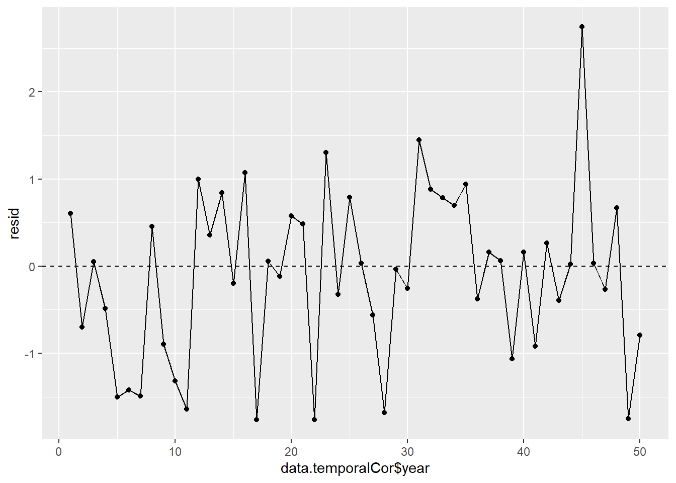

> 
> plot(acf(resid, lag = 40))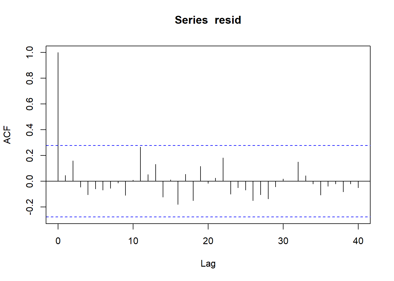

No obvious autocorrelation or other issues with residuals remaining.

Parameter estimates

Explore parameter estimates.

> library(broom)
> library(broom.mixed)
> tidyMCMC(as.mcmc(data.temporalCor.r2jags), conf.int = TRUE, conf.method = "HPDinterval")
# A tibble: 4 x 5
  term    estimate std.error conf.low conf.high
  <chr>      <dbl>     <dbl>    <dbl>     <dbl>
1 beta[1]   30.5     11.9      7.36      53.5  
2 beta[2]    0.225    0.100    0.0321     0.425
3 phi        0.919    0.0537   0.813      1.00 
4 sigma     12.0      1.25     9.91      14.7

Incorporating AR1 residual autocorrelation structure

Model fitting

> modelString2 = "
+   model {
+   #Likelihood
+   for (i in 1:n) {
+   mu[i] <- inprod(beta[],X[i,])
+   }
+   y[1:n] ~ dmnorm(mu[1:n],Omega)
+   for (i in 1:n) {
+   for (j in 1:n) {
+   Sigma[i,j] <- sigma2*(equals(i,j) + (1-equals(i,j))*pow(phi,abs(i-j))) 
+   }
+   }
+   Omega <- inverse(Sigma)
+   
+   #Priors
+   phi ~ dunif(-1,1)
+   for (i in 1:nX) {
+   beta[i] ~ dnorm(0,1.0E-6)
+   }
+   sigma <- z/sqrt(chSq)    # prior for sigma; cauchy = normal/sqrt(chi^2)
+   z ~ dnorm(0, 0.04)I(0,)
+   chSq ~ dgamma(0.5, 0.5)  # chi^2 with 1 d.f.
+   sigma2 = pow(sigma,2)
+   #tau.cor <- tau #* (1- phi*phi)
+   }
+   "
> 
> ## write the model to a text file
> writeLines(modelString2, con = "tempModel2.txt")

> Xmat = model.matrix(~x, data.temporalCor)
> data.temporalCor.list <- with(data.temporalCor, list(y = y, X = Xmat,
+     n = nrow(data.temporalCor), nX = ncol(Xmat)))

Define the nodes (parameters and derivatives) to monitor and the chain parameters.

> params <- c("beta", "sigma", "phi")
> nChains = 2
> burnInSteps = 5000
> thinSteps = 1
> numSavedSteps = 10000  #across all chains
> nIter = ceiling(burnInSteps + (numSavedSteps * thinSteps)/nChains)
> nIter
[1] 10000

Now run the JAGS code via the R2jags interface.

> data.temporalCor2.r2jags <- jags(data = data.temporalCor.list, inits = NULL, parameters.to.save = params,
+     model.file = "tempModel2.txt", n.chains = nChains, n.iter = nIter,
+     n.burnin = burnInSteps, n.thin = thinSteps)
Compiling model graph
   Resolving undeclared variables
   Allocating nodes
Graph information:
   Observed stochastic nodes: 1
   Unobserved stochastic nodes: 5
   Total graph size: 5566

Initializing model
> 
> print(data.temporalCor2.r2jags)
Inference for Bugs model at "tempModel2.txt", fit using jags,
 2 chains, each with 10000 iterations (first 5000 discarded)
 n.sims = 10000 iterations saved
         mu.vect sd.vect    2.5%     25%     50%     75%   97.5%  Rhat n.eff
beta[1]   19.926  24.597 -19.141   9.722  18.990  29.365  64.348 1.014 10000
beta[2]    0.225   0.100   0.028   0.159   0.227   0.291   0.421 1.001 10000
phi        0.890   0.055   0.773   0.854   0.895   0.930   0.980 1.011   160
sigma     30.352  15.780  18.171  22.799  26.810  32.951  61.419 1.010   410
deviance 392.642   2.706 389.232 390.628 392.029 394.019 399.490 1.001  2900

For each parameter, n.eff is a crude measure of effective sample size,
and Rhat is the potential scale reduction factor (at convergence, Rhat=1).

DIC info (using the rule, pD = var(deviance)/2)
pD = 3.7 and DIC = 396.3
DIC is an estimate of expected predictive error (lower deviance is better).

MCMC diagnostics

> denplot(data.temporalCor2.r2jags, parms = c("beta", "sigma", "phi"))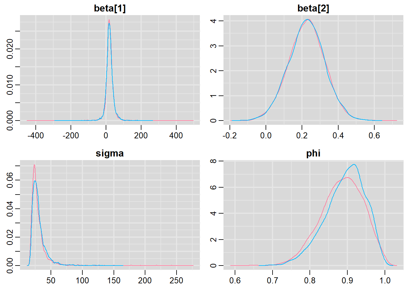

> traplot(data.temporalCor2.r2jags, parms = c("beta", "sigma", "phi"))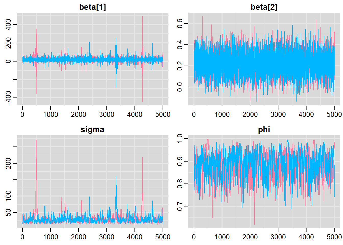

> data.mcmc = as.mcmc(data.temporalCor2.r2jags)
> #Raftery diagnostic
> raftery.diag(data.mcmc)
[[1]]

Quantile (q) = 0.025
Accuracy (r) = +/- 0.005
Probability (s) = 0.95 
                                                
          Burn-in  Total Lower bound  Dependence
          (M)      (N)   (Nmin)       factor (I)
 beta[1]  15       14982 3746         4.00      
 beta[2]  2        3866  3746         1.03      
 deviance 2        3995  3746         1.07      
 phi      9        9308  3746         2.48      
 sigma    8        10294 3746         2.75      


[[2]]

Quantile (q) = 0.025
Accuracy (r) = +/- 0.005
Probability (s) = 0.95 
                                                
          Burn-in  Total Lower bound  Dependence
          (M)      (N)   (Nmin)       factor (I)
 beta[1]  4        4955  3746         1.320     
 beta[2]  2        3620  3746         0.966     
 deviance 2        3930  3746         1.050     
 phi      12       12162 3746         3.250     
 sigma    8        10644 3746         2.840

> #Autocorrelation diagnostic
> autocorr.diag(data.mcmc)
            beta[1]      beta[2]   deviance       phi      sigma
Lag 0   1.000000000  1.000000000 1.00000000 1.0000000 1.00000000
Lag 1   0.023745389 -0.007088969 0.19477040 0.8775299 0.95206712
Lag 5   0.019171996  0.008569178 0.08589717 0.5774327 0.80961727
Lag 10 -0.009155805  0.008682983 0.06468974 0.3677587 0.64495814
Lag 50  0.012167974  0.014954099 0.01686647 0.0317406 0.04466731

All diagnostics seem fine.

Model validation

\[ Res_i = Y_i - \mu_i\]

\[ Res_{i+1} = Res_{i+1} - \rho Res_i\]

\[ Res_i = \frac{Res_i}{\sigma} \]

> mcmc = data.temporalCor2.r2jags$BUGSoutput$sims.matrix
> # generate a model matrix
> newdata = data.temporalCor
> Xmat = model.matrix(~x, newdata)
> ## get median parameter estimates
> wch = grep("beta", colnames(mcmc))
> coefs = mcmc[, wch]
> fit = coefs %*% t(Xmat)
> resid = -1 * sweep(fit, 2, data.temporalCor$y, "-")
> n = ncol(resid)
> resid[, -1] = resid[, -1] - (resid[, -n] * mcmc[, "phi"])
> resid = apply(resid, 2, median)/median(mcmc[, "sigma"])
> fit = apply(fit, 2, median)
> 
> ggplot() + geom_point(data = NULL, aes(y = resid, x = fit)) + theme_classic()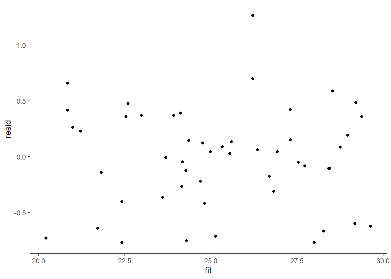

> 
> ggplot() + geom_point(data = NULL, aes(y = resid, x = data.temporalCor$x)) + theme_classic()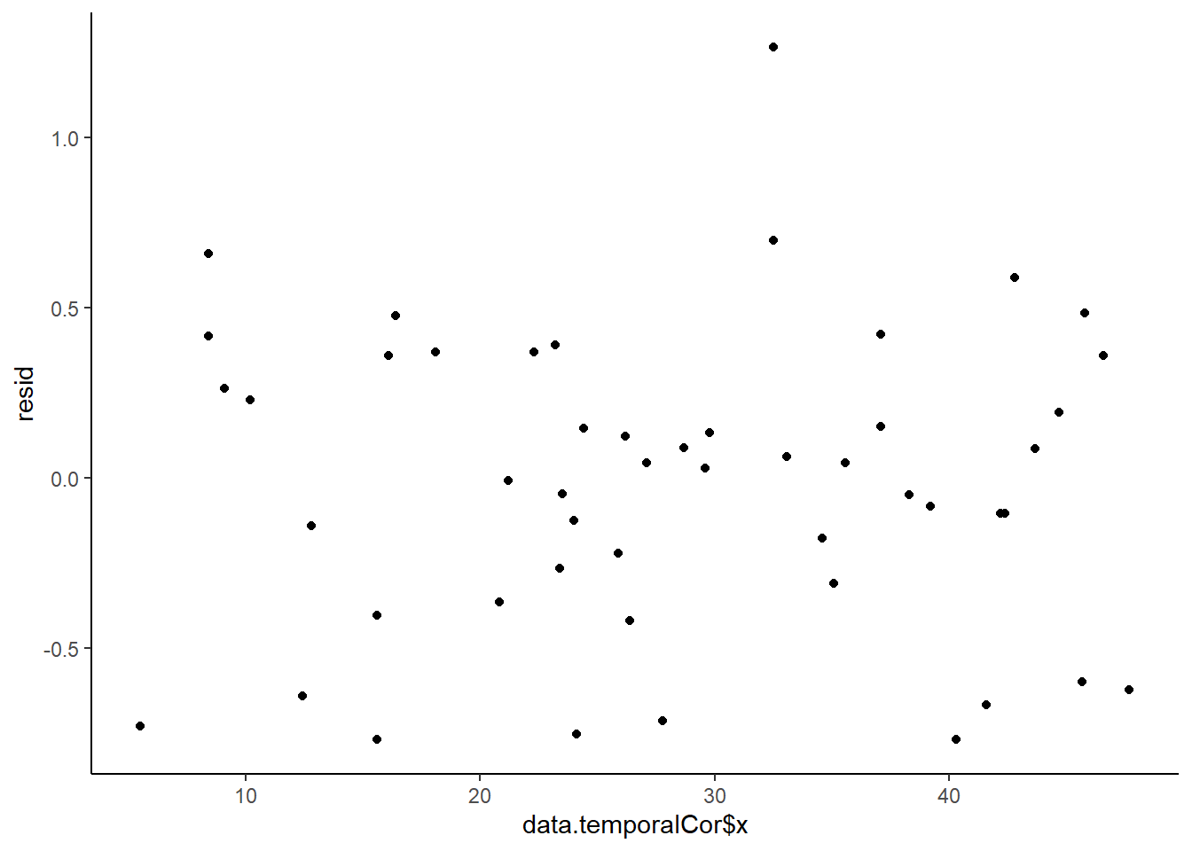

> 
> ggplot(data = NULL, aes(y = resid, x = data.temporalCor$year)) +
+     geom_point() + geom_line() + geom_hline(yintercept = 0, linetype = "dashed")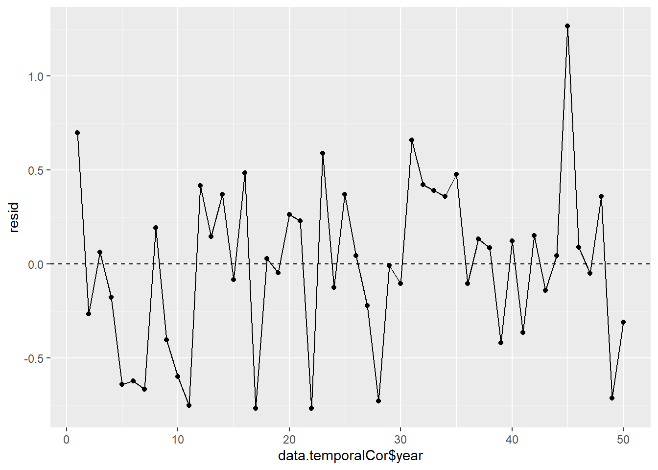

> 
> plot(acf(resid, lag = 40))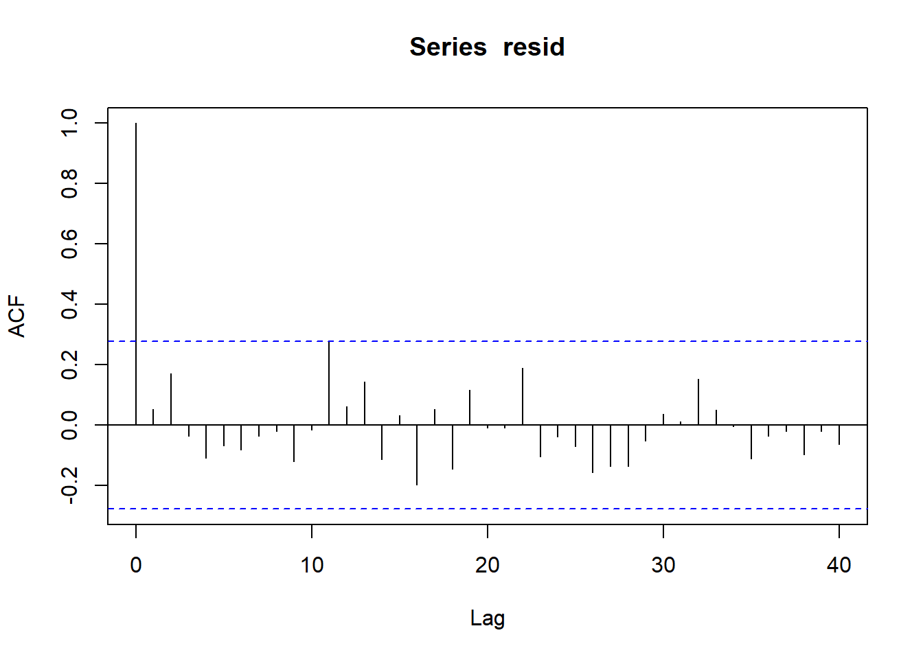

No obvious autocorrelation or other issues with residuals remaining

Parameter estimates

Explore parameter estimates.

> tidyMCMC(as.mcmc(data.temporalCor2.r2jags), conf.int = TRUE, conf.method = "HPDinterval")
# A tibble: 4 x 5
  term    estimate std.error conf.low conf.high
  <chr>      <dbl>     <dbl>    <dbl>     <dbl>
1 beta[1]   19.0     24.6    -16.6       66.3  
2 beta[2]    0.227    0.0997   0.0313     0.423
3 phi        0.895    0.0546   0.780      0.984
4 sigma     26.8     15.8     16.2       51.2

References

Plummer, Martyn. 2004. “JAGS: Just Another Gibbs Sampler.”

Su, Yu-Sung, Masanao Yajima, Maintainer Yu-Sung Su, and JAGS SystemRequirements. 2015. “Package ‘R2jags’.” R Package Version 0.03-08, URL Http://CRAN. R-Project. Org/Package= R2jags.

tutorials JAGS autocorrelation

Temporal Autocorrelation (JAGS)

Overview

Introduction

First order autocorrelation

Incorporating lagged residuals

Model fitting

MCMC diagnostics

Model validation

Parameter estimates

Incorporating AR1 residual autocorrelation structure

Model fitting

MCMC diagnostics

Model validation

Parameter estimates

References

Assistant Professor in Statistics