Temporal Autocorrelation (Stan)

Last updated on Feb 8, 2020 autocorrelation, Stan, R

This tutorial will focus on the use of Bayesian estimation to fit simple linear regression models. BUGS (Bayesian inference Using Gibbs Sampling) is an algorithm and supporting language (resembling R) dedicated to performing the Gibbs sampling implementation of Markov Chain Monte Carlo (MCMC) method. Dialects of the BUGS language are implemented within three main projects:

OpenBUGS - written in component pascal.
JAGS - (Just Another Gibbs Sampler) - written in C++.
Stan - a dedicated Bayesian modelling framework written in C++ and implementing Hamiltonian MCMC samplers.

Whilst the above programs can be used stand-alone, they do offer the rich data pre-processing and graphical capabilities of R, and thus, they are best accessed from within R itself. As such there are multiple packages devoted to interfacing with the various software implementations:

R2OpenBUGS - interfaces with OpenBUGS
R2jags - interfaces with JAGS
rstan - interfaces with Stan

This tutorial will demonstrate how to fit models in Stan (Gelman, Lee, and Guo (2015)) using the package rstan (Stan Development Team (2018)) as interface, which also requires to load some other packages.

Overview

Introduction

Up until now (in the proceeding tutorials), the focus has been on models that adhere to specific assumptions about the underlying populations (and data). Indeed, both before and immediately after fitting these models, I have stressed the importance of evaluating and validating the proposed and fitted models to ensure reliability of the models. It is now worth us revisiting those fundamental assumptions as well as exploring the options that are available when the populations (data) do not conform. Let’s explore a simple linear regression model to see how each of the assumptions relate to the model.

\[ y_i = \beta_0 + \beta_1x_i + \epsilon_i \;\;\; \text{with} \;\;\; \epsilon_i \sim \text{Normal}(0, \sigma^2).\]

The above simple statistical model models the linear relationship of \(y_i\) against \(x_i\). The residuals (\(\epsilon\)) are assumed to be normally distributed with a mean of zero and a constant (yet unknown) variance (\(\sigma\), homogeneity of variance). The residuals (and thus observations) are also assumed to all be independent.

Homogeneity of variance and independence are encapsulated within the single symbol for variance (\(\sigma^2\)). In assuming equal variances and independence, we are actually making an assumption about the variance-covariance structure of the populations (and thus residuals). Specifically, we assume that all populations are equally varied and thus can be represented well by a single variance term (all diagonal values in a \(N\times N\) covariance matrix are the same, \(\sigma^2\)) and the covariances between each population are zero (off diagonals). In simple regression, each observation (data point) represents a single observation drawn (sampled) from an entire population of possible observations. The above covariance structure thus assumes that the covariance between each population (observation) is zero - that is, each observation is completely independent of each other observation. Whilst it is mathematically convenient when data conform to these conditions (normality, homogeneity of variance, independence and linearity), data often violate one or more of these assumptions. In the following, I want to discuss and explore the causes and options for dealing with non-compliance to each of these conditions. By gaining a better understanding of how the various model fitting engines perform their task, we are better equipped to accommodate aspects of the data that don’t otherwise conform to the simple regression assumptions. In this tutorial we specifically focus on the topic of heterogeneity of the variance.

In order that the estimated parameters represent the underlying populations in an unbiased manner, the residuals (and thus each each observation) must be independent. However, what if we were sampling a population over time and we were interested in investigating how changes in a response relate to changes in a predictor (such as rainfall). For any response that does not “reset” itself on a regular basis, the state of the population (the value of its response) at a given time is likely to be at least partly dependent on the state of the population at the sampling time before. We can further generalise the above into:

\[ y_i \sim Dist(\mu_i),\]

where \(\mu_i=\boldsymbol X \boldsymbol \beta + \boldsymbol Z \boldsymbol \gamma\), with \(\boldsymbol X\) and \(\boldsymbol \beta\) representing the fixed data structure and fixed effects, respectively, while with \(\boldsymbol Z\) and \(\boldsymbol \gamma\) represent the varying data structure and varying effects, respectively. In simple regression, there are no “varying” effects, and thus:

\[ \boldsymbol \gamma \sim MVN(\boldsymbol 0, \boldsymbol \Sigma),\]

where \(\boldsymbol \Sigma\) is a variance-covariance matrix of the form

\[ \boldsymbol \Sigma = \frac{\sigma^2}{1-\rho^2} \begin{bmatrix} 1 & \rho^{\phi_{1,2}} & \ldots & \rho^{\phi_{1,n}} \\ \rho^{\phi_{2,1}} & 1 & \ldots & \vdots\\ \vdots & \ldots & 1 & \vdots\\ \rho^{\phi_{n,1}} & \ldots & \ldots & 1 \end{bmatrix}. \]

Notice that this introduces a very large number of additional parameters that require estimating: \(\sigma^2\) (error variance), \(\rho\) (base autocorrelation) and each of the individual covariances (\(\rho^{\phi_{n,n}}\)). Hence, there are always going to be more parameters to estimate than there are date avaiable to use to estimate these paramters. We typically make one of a number of alternative assumptions so as to make this task more manageable.

When we assume that all residuals are independent (regular regression), i.e. \(\rho=0\), \(\boldsymbol \Sigma\) is essentially equal to \(\sigma^2 \boldsymbol I\) and we simply use:

\[ \boldsymbol \gamma \sim N( 0,\sigma^2).\]

We could assume there is a reasonably simple pattern of correlation that declines over time. The simplest of these is a first order autoregressive (AR1) structure in which exponent on the correlation declines linearly according to the time lag (\(\mid t - s\mid\)).

\[ \boldsymbol \Sigma = \frac{\sigma^2}{1-\rho^2} \begin{bmatrix} 1 & \rho & \ldots & \rho^{\mid t-s \mid} \\ \rho & 1 & \ldots & \vdots\\ \vdots & \ldots & 1 & \vdots\\ \rho^{\mid t-s \mid } & \ldots & \ldots & 1 \end{bmatrix}. \]

Note, in making this assumption, we are also assuming that the degree of correlation is dependent only on the lag and not on when the lag occurs (stationarity). That is all lag 1 residual pairs will have the same degree of correlation, all the lag \(2\) pairs will have the same correlation and so on.

First order autocorrelation

Consider an example, in which the number of individuals at time \(2\) will be partly dependent on the number of individuals present at time \(1\). Clearly then, the observations (and thus residuals) are not fully independent - there is an auto-regressive correlation dependency structure. We could accommodate this lack of independence by fitting a model that incorporates a AR1 variance-covariance structure. Alternatively, we fit the following model:

\[ y_{it} \sim Dist(\mu_{it}),\]

where

\[\mu_{it}=\boldsymbol X \boldsymbol \beta + \rho \epsilon_{i,t-1} + \gamma_{it},\]

and where \(\gamma \sim N(0, \sigma^2)\). In this version of the model, we are stating that the expected value of an observation is equal to the regular linear predictor plus the autocorrelation parameter (\(\rho\)) multipled by the residual associated with the previous observation plus the regular independently distributed noise (\(\sigma^2\)). Such a model is substantially faster to fit, although along with stationarity assumes in estimating the autocorrelation parameter, only the smallest lags are used. To see this in action, we will first generate some temporally auto-correlated data.

> set.seed(126)
> n = 50
> a <- 20  #intercept
> b <- 0.2  #slope
> x <- round(runif(n, 1, n), 1)  #values of the year covariate
> year <- 1:n
> sigma <- 20
> rho <- 0.8
> 
> library(nlme)
> ## define a constructor for a first-order
> ## correlation structure
> ar1 <- corAR1(form = ~year, value = rho)
> ## initialize this constructor against our data
> AR1 <- Initialize(ar1, data = data.frame(year))
> ## generate a correlation matrix
> V <- corMatrix(AR1)
> ## Cholesky factorization of V
> Cv <- chol(V)
> ## simulate AR1 errors
> e <- t(Cv) %*% rnorm(n, 0, sigma)  # cov(e) = V * sig^2
> ## generate response
> y <- a + b * x + e
> data.temporalCor = data.frame(y = y, x = x, year = year)
> write.table(data.temporalCor, file = "data.temporalCor.csv",
+     sep = ",", quote = F, row.names = FALSE)
> 
> pairs(data.temporalCor)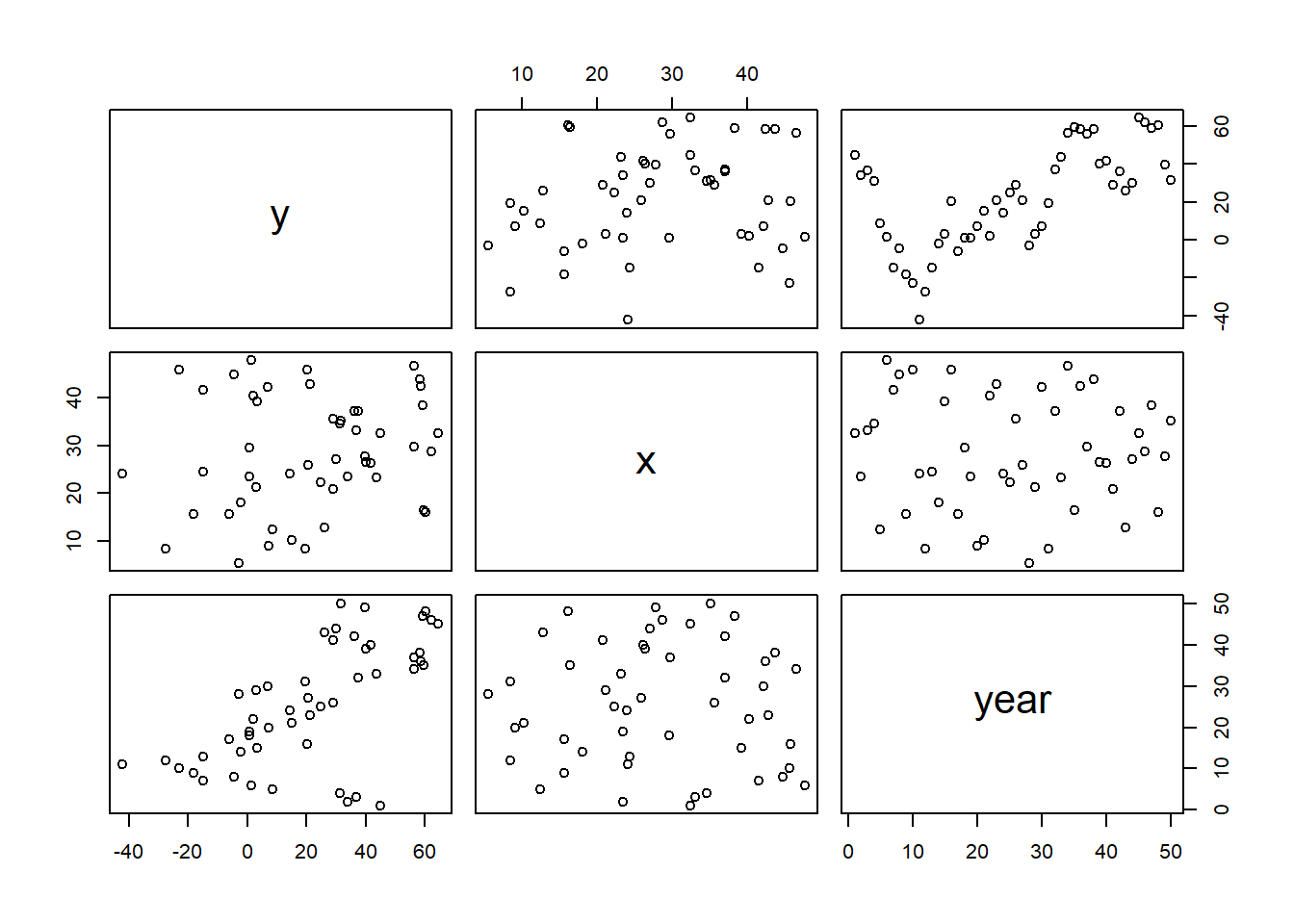

We will now proceed to analyse these data via both of the above techniques for JAGS:

incorporating AR1 residual autocorrelation structure
incorporating lagged residuals into the model

Incorporating lagged residuals

Model fitting

We proceed to code the model into JAGS (remember that in this software normal distribution are parameterised in terms of precisions \(\tau\) rather than variances, where \(\tau=\frac{1}{\sigma^2}\)). Define the model.

> stanString = "
+   data {
+   int<lower=1> n;
+   vector [n] y;
+   int<lower=1> nX;
+   matrix[n,nX] X;
+   }
+   transformed data {
+   }
+   parameters {
+   vector[nX] beta;
+   real<lower=0> sigma;
+   real<lower=-1,upper=1> phi;
+   }
+   transformed parameters {
+   vector[n] mu;
+   vector[n] epsilon;
+   mu = X*beta;
+   epsilon[1] = y[1] - mu[1];
+   for (i in 2:n) {
+   epsilon[i] = (y[i] - mu[i]);
+   mu[i] = mu[i] + phi*epsilon[i-1];
+   }
+   }
+   model {
+   phi ~ uniform(-1,1);
+   beta ~ normal(0,100);
+   sigma ~ cauchy(0,5);
+   y ~ normal(mu, sigma);
+   }
+   generated quantities {
+   }
+   
+   "
> 
> ## write the model to a text file
> writeLines(stanString, con = "tempModel.stan")

Arrange the data as a list (as required by Stan). As input, Stan will need to be supplied with: the response variable, the predictor variable, the total number of observed items. This all needs to be contained within a list object. We will create two data lists, one for each of the hypotheses.

> Xmat = model.matrix(~x, data.temporalCor)
> data.temporalCor.list <- with(data.temporalCor, list(y = y, X = Xmat,
+     n = nrow(data.temporalCor), nX = ncol(Xmat)))

Define the nodes (parameters and derivatives) to monitor and chain parameters.

> params <- c("beta", "sigma", "phi")
> nChains = 2
> burnInSteps = 500
> thinSteps = 1
> numSavedSteps = 2000  #across all chains
> nIter = ceiling(burnInSteps + (numSavedSteps * thinSteps)/nChains)
> nIter
[1] 1500

Now compile and run the Stan code via the rstan interface.

> library(rstan)

During the warmup stage, the No-U-Turn sampler (NUTS) attempts to determine the optimum stepsize - the stepsize that achieves the target acceptance rate (\(0.8\) or \(80\)% by default) without divergence (occurs when the stepsize is too large relative to the curvature of the log posterior and results in approximations that are likely to diverge and be biased) - and without hitting the maximum treedepth (\(10\)). At each iteration of the NUTS algorithm, the number of leapfrog steps doubles (as it increases the treedepth) and only terminates when either the NUTS criterion are satisfied or the tree depth reaches the maximum (\(10\) by default).

> data.temporalCor.rstan <- stan(data = data.temporalCor.list, file = "tempModel.stan", chains = nChains, pars = params, iter = nIter, warmup = burnInSteps, thin = thinSteps)

SAMPLING FOR MODEL 'tempModel' NOW (CHAIN 1).
Chain 1: 
Chain 1: Gradient evaluation took 0 seconds
Chain 1: 1000 transitions using 10 leapfrog steps per transition would take 0 seconds.
Chain 1: Adjust your expectations accordingly!
Chain 1: 
Chain 1: 
Chain 1: Iteration:    1 / 1500 [  0%]  (Warmup)
Chain 1: Iteration:  150 / 1500 [ 10%]  (Warmup)
Chain 1: Iteration:  300 / 1500 [ 20%]  (Warmup)
Chain 1: Iteration:  450 / 1500 [ 30%]  (Warmup)
Chain 1: Iteration:  501 / 1500 [ 33%]  (Sampling)
Chain 1: Iteration:  650 / 1500 [ 43%]  (Sampling)
Chain 1: Iteration:  800 / 1500 [ 53%]  (Sampling)
Chain 1: Iteration:  950 / 1500 [ 63%]  (Sampling)
Chain 1: Iteration: 1100 / 1500 [ 73%]  (Sampling)
Chain 1: Iteration: 1250 / 1500 [ 83%]  (Sampling)
Chain 1: Iteration: 1400 / 1500 [ 93%]  (Sampling)
Chain 1: Iteration: 1500 / 1500 [100%]  (Sampling)
Chain 1: 
Chain 1:  Elapsed Time: 0.125 seconds (Warm-up)
Chain 1:                0.127 seconds (Sampling)
Chain 1:                0.252 seconds (Total)
Chain 1: 

SAMPLING FOR MODEL 'tempModel' NOW (CHAIN 2).
Chain 2: 
Chain 2: Gradient evaluation took 0 seconds
Chain 2: 1000 transitions using 10 leapfrog steps per transition would take 0 seconds.
Chain 2: Adjust your expectations accordingly!
Chain 2: 
Chain 2: 
Chain 2: Iteration:    1 / 1500 [  0%]  (Warmup)
Chain 2: Iteration:  150 / 1500 [ 10%]  (Warmup)
Chain 2: Iteration:  300 / 1500 [ 20%]  (Warmup)
Chain 2: Iteration:  450 / 1500 [ 30%]  (Warmup)
Chain 2: Iteration:  501 / 1500 [ 33%]  (Sampling)
Chain 2: Iteration:  650 / 1500 [ 43%]  (Sampling)
Chain 2: Iteration:  800 / 1500 [ 53%]  (Sampling)
Chain 2: Iteration:  950 / 1500 [ 63%]  (Sampling)
Chain 2: Iteration: 1100 / 1500 [ 73%]  (Sampling)
Chain 2: Iteration: 1250 / 1500 [ 83%]  (Sampling)
Chain 2: Iteration: 1400 / 1500 [ 93%]  (Sampling)
Chain 2: Iteration: 1500 / 1500 [100%]  (Sampling)
Chain 2: 
Chain 2:  Elapsed Time: 0.138 seconds (Warm-up)
Chain 2:                0.153 seconds (Sampling)
Chain 2:                0.291 seconds (Total)
Chain 2: 
> 
> print(data.temporalCor.rstan, par = c("beta", "sigma", "phi"))
Inference for Stan model: tempModel.
2 chains, each with iter=1500; warmup=500; thin=1; 
post-warmup draws per chain=1000, total post-warmup draws=2000.

         mean se_mean    sd  2.5%   25%   50%   75% 97.5% n_eff Rhat
beta[1] 29.72    0.32 11.50  8.41 21.73 29.47 37.24 53.73  1298    1
beta[2]  0.23    0.00  0.10  0.04  0.16  0.23  0.29  0.42  1104    1
sigma   12.03    0.03  1.20 10.03 11.13 11.95 12.79 14.57  1281    1
phi      0.91    0.00  0.05  0.79  0.88  0.91  0.95  0.99  1150    1

Samples were drawn using NUTS(diag_e) at Thu Jul 08 20:41:31 2021.
For each parameter, n_eff is a crude measure of effective sample size,
and Rhat is the potential scale reduction factor on split chains (at 
convergence, Rhat=1).

MCMC diagnostics

> library(mcmcplots)
> mcmc = As.mcmc.list(data.temporalCor.rstan)
> denplot(mcmc, parms = c("beta", "sigma", "phi"))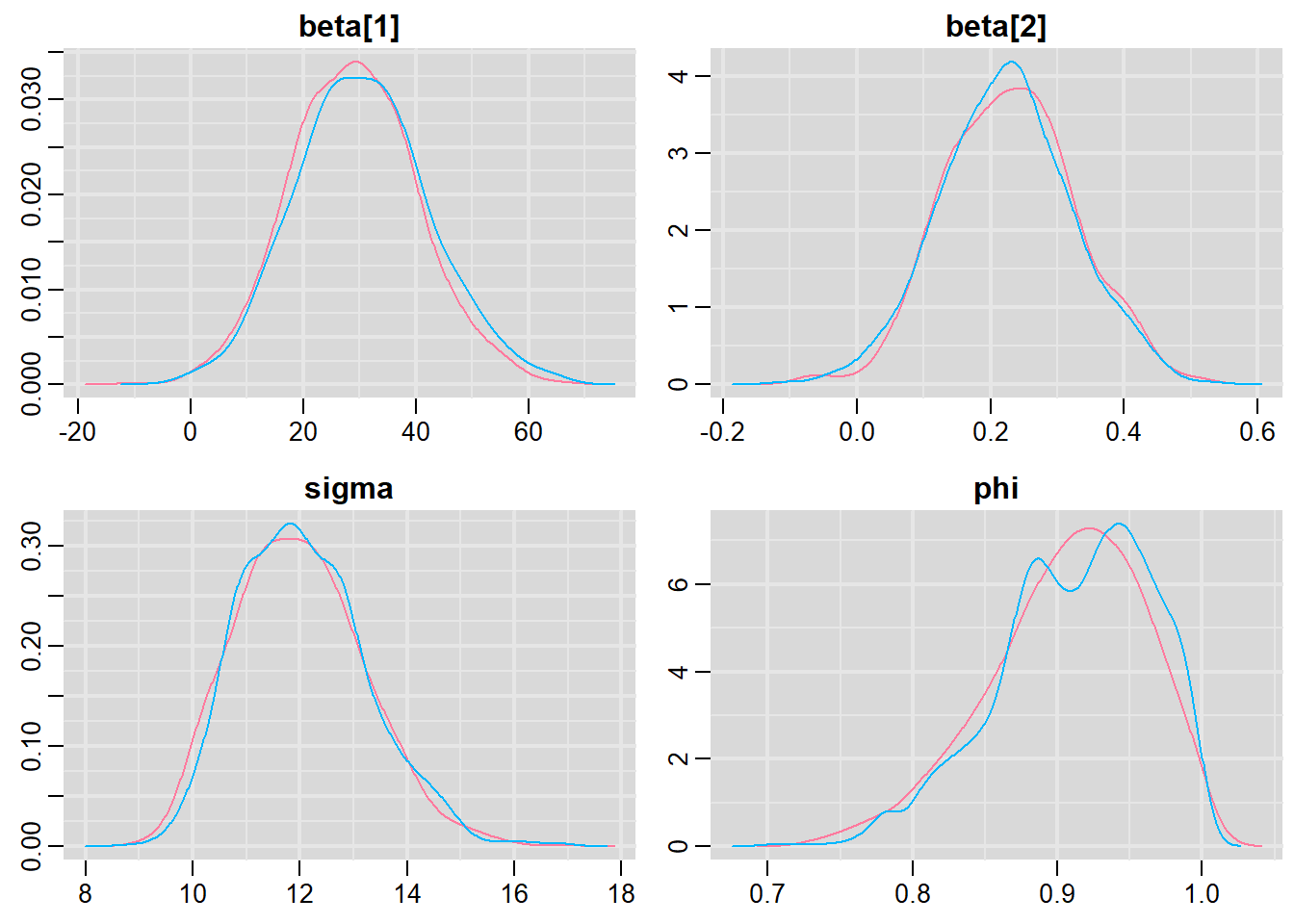

> traplot(mcmc, parms = c("beta", "sigma", "phi"))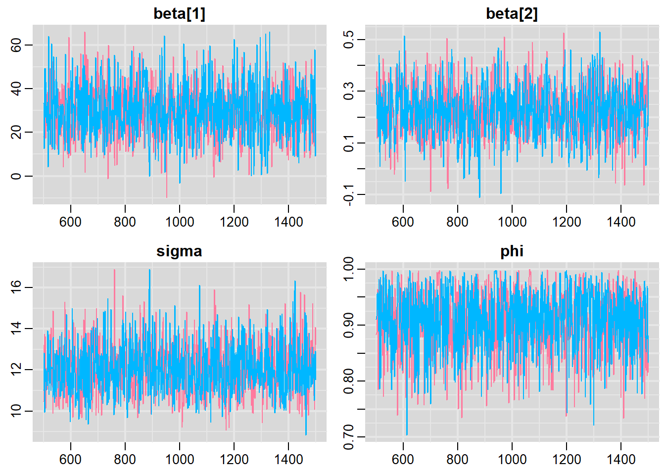

> #Raftery diagnostic
> raftery.diag(mcmc)
[[1]]

Quantile (q) = 0.025
Accuracy (r) = +/- 0.005
Probability (s) = 0.95 

You need a sample size of at least 3746 with these values of q, r and s

[[2]]

Quantile (q) = 0.025
Accuracy (r) = +/- 0.005
Probability (s) = 0.95 

You need a sample size of at least 3746 with these values of q, r and s

> #Autocorrelation diagnostic
> autocorr.diag(mcmc)
           beta[1]       beta[2]       sigma         phi         lp__
Lag 0   1.00000000  1.0000000000  1.00000000  1.00000000  1.000000000
Lag 1   0.21294298  0.2877759622  0.21935566  0.08690846  0.428661908
Lag 5  -0.04138775 -0.0210755053 -0.01868804  0.07309205  0.024806402
Lag 10  0.01829666  0.0195631851  0.01665466 -0.01348082  0.002269007
Lag 50 -0.00781781 -0.0006062359  0.01350526 -0.02697167 -0.038734864

> stan_ac(data.temporalCor.rstan)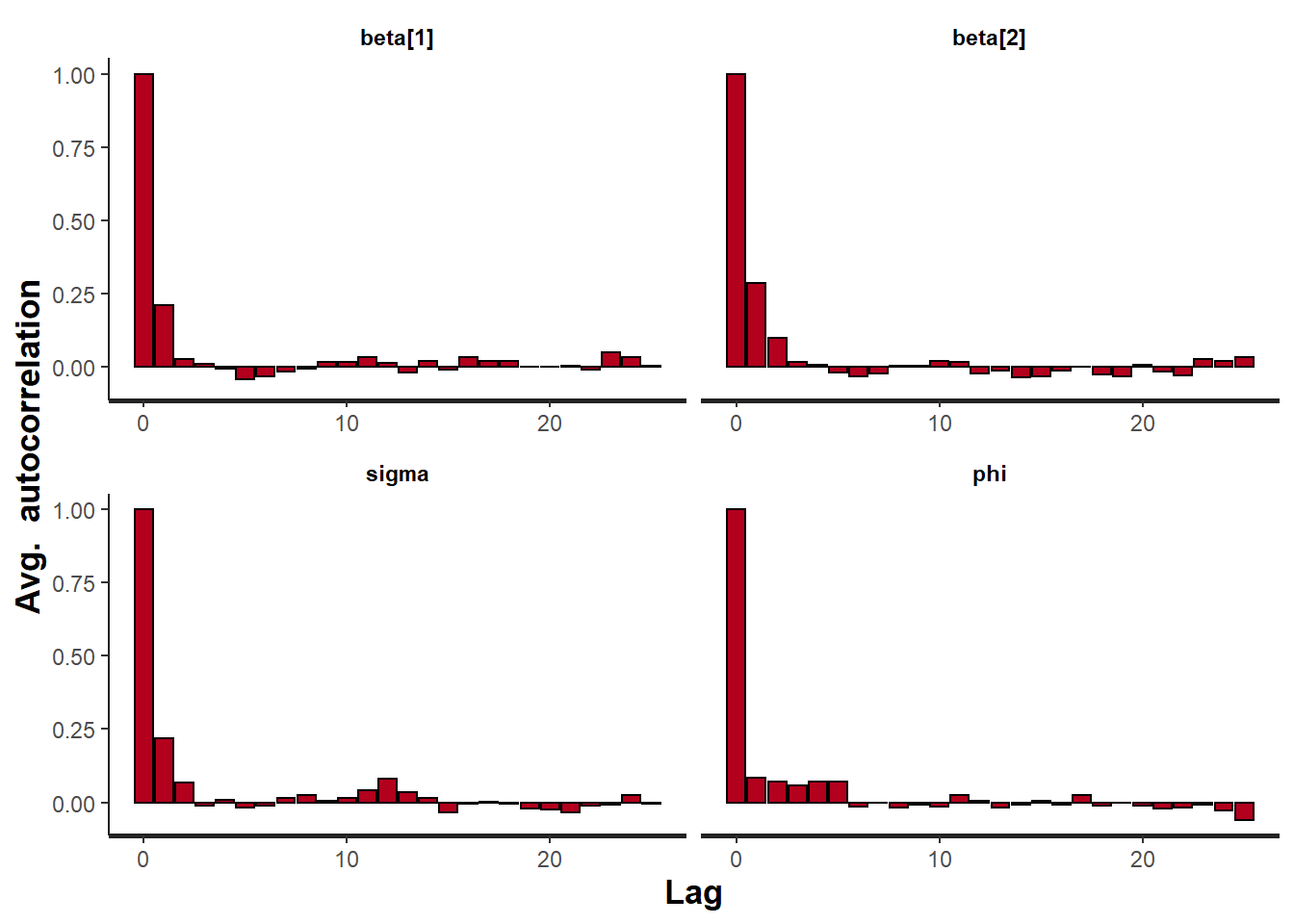

> stan_rhat(data.temporalCor.rstan)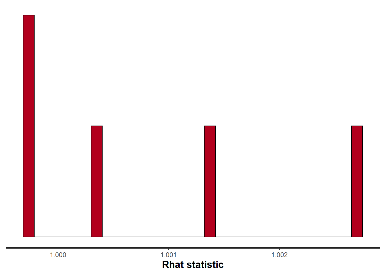

> stan_ess(data.temporalCor.rstan)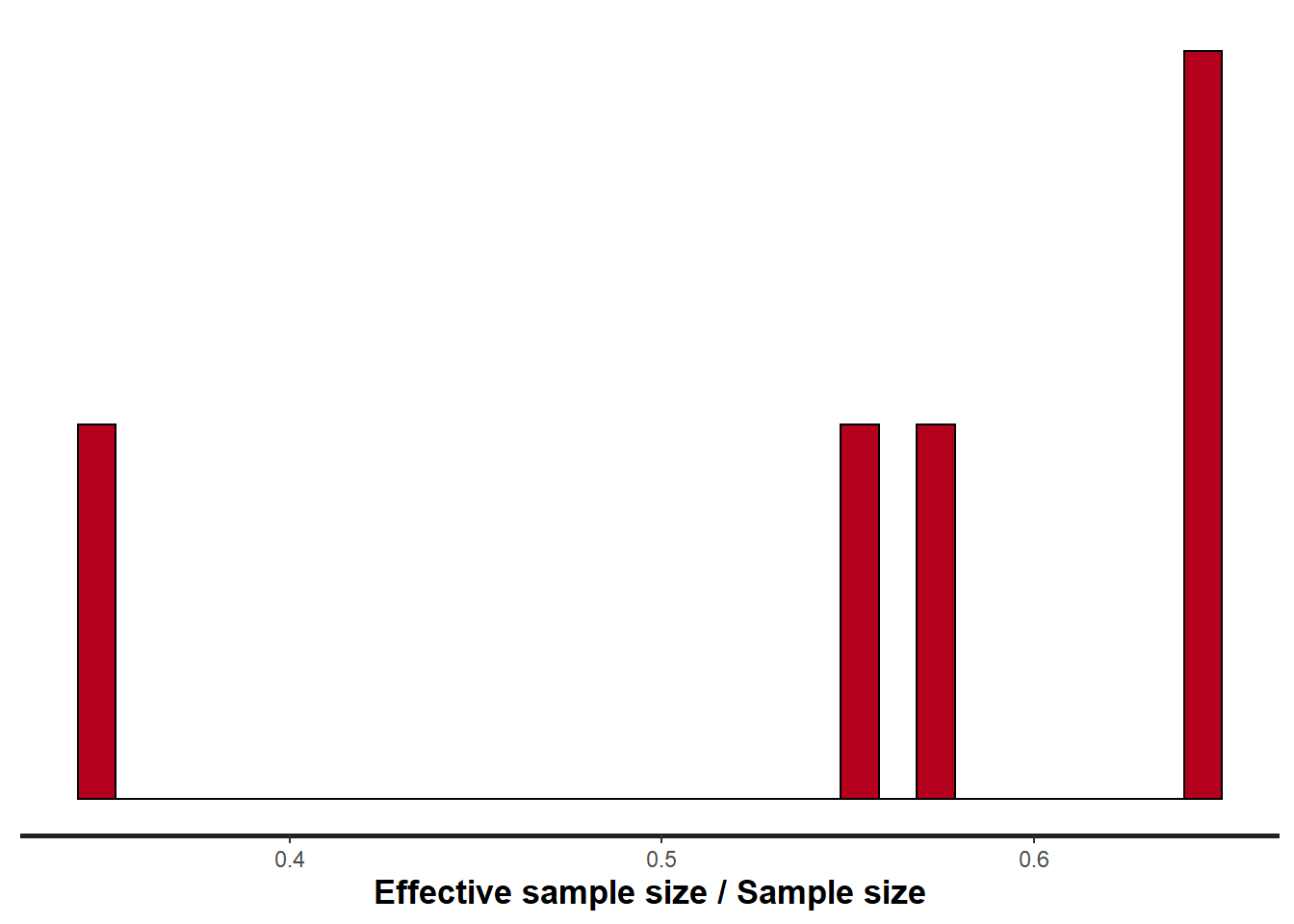

All diagnostics seem fine.

Model validation

Whenever we fit a model that incorporates changes to the variance-covariance structures, we need to explore modified standardized residuals. In this case, the raw residuals should be updated to reflect the autocorrelation (subtract residual from previous time weighted by the autocorrelation parameter) before standardising by sigma.

\[ Res_i = Y_i - \mu_i\]

\[ Res_{i+1} = Res_{i+1} - \rho Res_i\]

\[ Res_i = \frac{Res_i}{\sigma} \]

> mcmc = as.matrix(data.temporalCor.rstan)
> wch = grep("beta", colnames(mcmc))
> # generate a model matrix
> newdata = data.frame(x = data.temporalCor$x)
> Xmat = model.matrix(~x, newdata)
> ## get median parameter estimates
> coefs = mcmc[, wch]
> fit = coefs %*% t(Xmat)
> resid = -1 * sweep(fit, 2, data.temporalCor$y, "-")
> n = ncol(resid)
> resid[, -1] = resid[, -1] - (resid[, -n] * mcmc[, "phi"])
> resid = apply(resid, 2, median)/median(mcmc[, "sigma"])
> fit = apply(fit, 2, median)
> 
> library(ggplot2)
> ggplot() + geom_point(data = NULL, aes(y = resid, x = fit)) + theme_classic()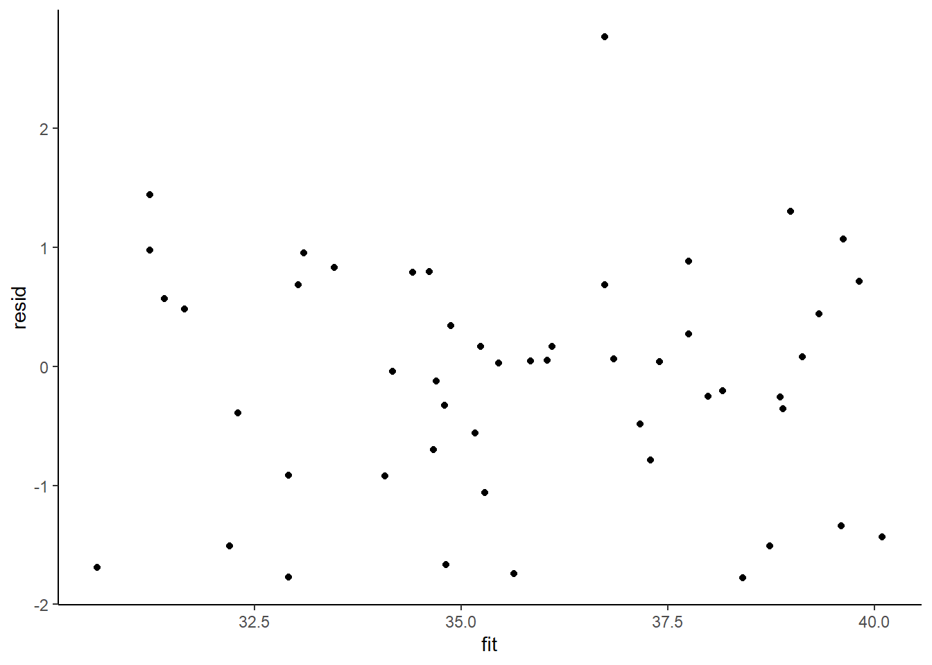

> 
> ggplot() + geom_point(data = NULL, aes(y = resid, x = data.temporalCor$x)) + theme_classic()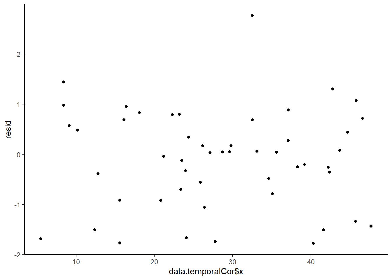

> 
> ggplot(data = NULL, aes(y = resid, x = data.temporalCor$year)) +
+     geom_point() + geom_line() + geom_hline(yintercept = 0, linetype = "dashed") + theme_classic()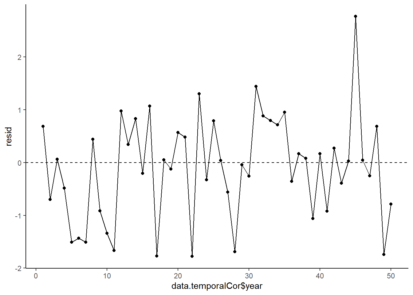

> 
> plot(acf(resid, lag = 40))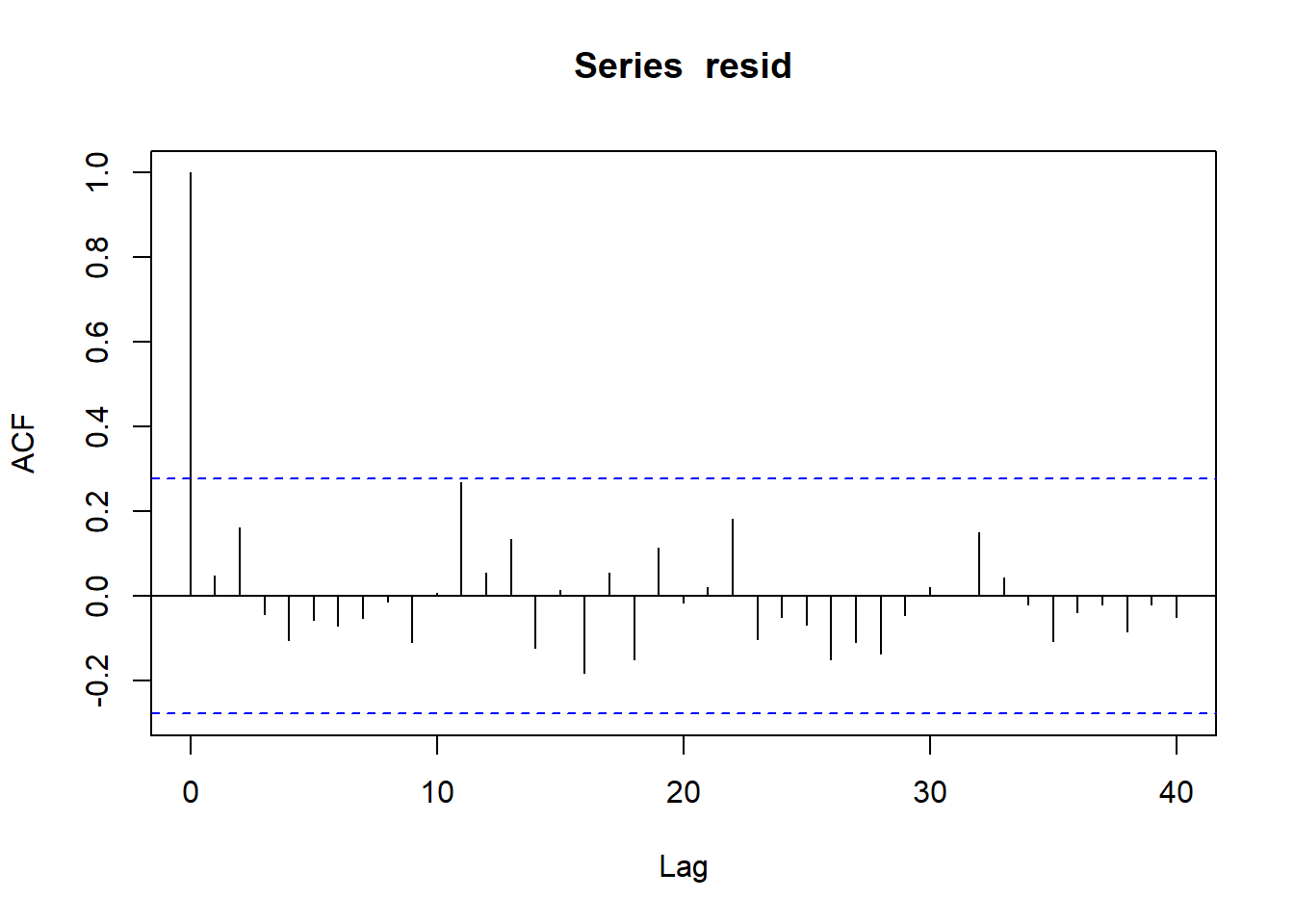

> 
> fit = coefs %*% t(Xmat)
> ## draw samples from this model
> yRep = sapply(1:nrow(mcmc), function(i) rnorm(nrow(data.temporalCor),
+     fit[i, ], mcmc[i, "sigma"]))
> ggplot() + geom_density(data = NULL, aes(x = as.vector(yRep),
+     fill = "Model"), alpha = 0.5) + geom_density(data = data.temporalCor,
+     aes(x = y, fill = "Obs"), alpha = 0.5) + theme_classic()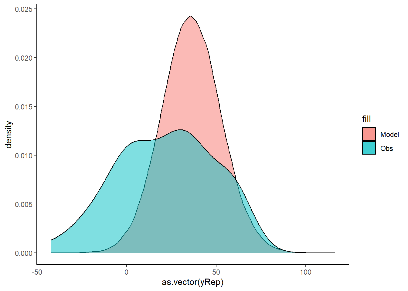

No obvious autocorrelation or other issues with residuals remaining.

Parameter estimates

Explore parameter estimates.

> library(broom)
> library(broom.mixed)
> tidyMCMC(data.temporalCor.rstan, par = c("beta", "phi", "sigma"),
+     conf.int = TRUE, conf.method = "HPDinterval", rhat = TRUE,
+     ess = TRUE)
# A tibble: 4 x 7
  term    estimate std.error conf.low conf.high  rhat   ess
  <chr>      <dbl>     <dbl>    <dbl>     <dbl> <dbl> <int>
1 beta[1]   29.5     11.5      8.62      53.9    1.00  1298
2 beta[2]    0.225    0.0980   0.0435     0.422  1.00  1104
3 phi        0.915    0.0533   0.809      0.998  1.00  1150
4 sigma     12.0      1.20     9.88      14.3    1.00  1281

Incorporating AR1 residual autocorrelation structure

Model fitting

> stanString = "
+ functions { 
+   matrix cov_matrix_ar1(real ar, real sigma, int nrows) { 
+   matrix[nrows, nrows] mat; 
+   vector[nrows - 1] gamma; 
+   mat = diag_matrix(rep_vector(1, nrows)); 
+       for (i in 2:nrows) { 
+           gamma[i - 1] = pow(ar, i - 1); 
+               for (j in 1:(i - 1)) { 
+                       mat[i, j] = gamma[i - j]; 
+                       mat[j, i] = gamma[i - j]; 
+                   } 
+               } 
+               return sigma^2 / (1 - ar^2) * mat; 
+       }
+ } 
+     
+       data { 
+            int<lower=1> n;  // total number of observations 
+                vector[n] y;  // response variable
+                int<lower=1> nX;
+                    matrix[n,nX] X;
+          } 
+            transformed data {
+               vector[n] se2 = rep_vector(0, n); 
+            } 
+            parameters { 
+               vector[nX] beta;
+                   real<lower=0> sigma;  // residual SD 
+                   real <lower=-1,upper=1> phi;  // autoregressive effects 
+               } 
+               transformed parameters { 
+               } 
+               model {
+                   matrix[n, n] res_cov_matrix;
+                   matrix[n, n] Sigma; 
+                   vector[n] mu = X*beta;
+                   res_cov_matrix = cov_matrix_ar1(phi, sigma, n);
+                   Sigma = res_cov_matrix + diag_matrix(se2);
+                   Sigma = cholesky_decompose(Sigma); 
+ 
+                   // priors including all constants
+                   beta ~ student_t(3,30,30);
+                   sigma ~ cauchy(0,5);
+                   y ~ multi_normal_cholesky(mu,Sigma);
+               } 
+               generated quantities { 
+               }
+   
+   "
> 
> ## write the model to a text file
> writeLines(stanString, con = "tempModel2.stan")

> Xmat = model.matrix(~x, data.temporalCor)
> data.temporalCor.list <- with(data.temporalCor, list(y = y, X = Xmat,
+     n = nrow(data.temporalCor), nX = ncol(Xmat)))

Define the nodes (parameters and derivatives) to monitor and chain parameters.

> params <- c("beta", "sigma", "phi")
> nChains = 2
> burnInSteps = 500
> thinSteps = 1
> numSavedSteps = 2000  #across all chains
> nIter = ceiling(burnInSteps + (numSavedSteps * thinSteps)/nChains)
> nIter
[1] 1500

Now compile and run the Stan code via the rstan interface.

> data.temporalCor2.rstan <- stan(data = data.temporalCor.list, file = "tempModel2.stan", chains = nChains, pars = params, iter = nIter, warmup = burnInSteps, thin = thinSteps)

SAMPLING FOR MODEL 'tempModel2' NOW (CHAIN 1).
Chain 1: 
Chain 1: Gradient evaluation took 0.001 seconds
Chain 1: 1000 transitions using 10 leapfrog steps per transition would take 10 seconds.
Chain 1: Adjust your expectations accordingly!
Chain 1: 
Chain 1: 
Chain 1: Iteration:    1 / 1500 [  0%]  (Warmup)
Chain 1: Iteration:  150 / 1500 [ 10%]  (Warmup)
Chain 1: Iteration:  300 / 1500 [ 20%]  (Warmup)
Chain 1: Iteration:  450 / 1500 [ 30%]  (Warmup)
Chain 1: Iteration:  501 / 1500 [ 33%]  (Sampling)
Chain 1: Iteration:  650 / 1500 [ 43%]  (Sampling)
Chain 1: Iteration:  800 / 1500 [ 53%]  (Sampling)
Chain 1: Iteration:  950 / 1500 [ 63%]  (Sampling)
Chain 1: Iteration: 1100 / 1500 [ 73%]  (Sampling)
Chain 1: Iteration: 1250 / 1500 [ 83%]  (Sampling)
Chain 1: Iteration: 1400 / 1500 [ 93%]  (Sampling)
Chain 1: Iteration: 1500 / 1500 [100%]  (Sampling)
Chain 1: 
Chain 1:  Elapsed Time: 4.945 seconds (Warm-up)
Chain 1:                2.9 seconds (Sampling)
Chain 1:                7.845 seconds (Total)
Chain 1: 

SAMPLING FOR MODEL 'tempModel2' NOW (CHAIN 2).
Chain 2: 
Chain 2: Gradient evaluation took 0 seconds
Chain 2: 1000 transitions using 10 leapfrog steps per transition would take 0 seconds.
Chain 2: Adjust your expectations accordingly!
Chain 2: 
Chain 2: 
Chain 2: Iteration:    1 / 1500 [  0%]  (Warmup)
Chain 2: Iteration:  150 / 1500 [ 10%]  (Warmup)
Chain 2: Iteration:  300 / 1500 [ 20%]  (Warmup)
Chain 2: Iteration:  450 / 1500 [ 30%]  (Warmup)
Chain 2: Iteration:  501 / 1500 [ 33%]  (Sampling)
Chain 2: Iteration:  650 / 1500 [ 43%]  (Sampling)
Chain 2: Iteration:  800 / 1500 [ 53%]  (Sampling)
Chain 2: Iteration:  950 / 1500 [ 63%]  (Sampling)
Chain 2: Iteration: 1100 / 1500 [ 73%]  (Sampling)
Chain 2: Iteration: 1250 / 1500 [ 83%]  (Sampling)
Chain 2: Iteration: 1400 / 1500 [ 93%]  (Sampling)
Chain 2: Iteration: 1500 / 1500 [100%]  (Sampling)
Chain 2: 
Chain 2:  Elapsed Time: 4.756 seconds (Warm-up)
Chain 2:                3.1 seconds (Sampling)
Chain 2:                7.856 seconds (Total)
Chain 2: 
> 
> print(data.temporalCor2.rstan, par = c("beta", "sigma", "phi"))
Inference for Stan model: tempModel2.
2 chains, each with iter=1500; warmup=500; thin=1; 
post-warmup draws per chain=1000, total post-warmup draws=2000.

         mean se_mean    sd  2.5%   25%   50%   75% 97.5% n_eff Rhat
beta[1] 22.23    0.42 15.12 -6.91 13.08 21.88 30.86 54.26  1321    1
beta[2]  0.22    0.00  0.10  0.04  0.16  0.22  0.29  0.42  1220    1
sigma   11.98    0.03  1.23  9.85 11.11 11.88 12.79 14.66  1659    1
phi      0.90    0.00  0.06  0.78  0.86  0.90  0.94  0.98  1355    1

Samples were drawn using NUTS(diag_e) at Thu Jul 08 20:42:34 2021.
For each parameter, n_eff is a crude measure of effective sample size,
and Rhat is the potential scale reduction factor on split chains (at 
convergence, Rhat=1).

MCMC diagnostics

> mcmc = As.mcmc.list(data.temporalCor2.rstan)
> denplot(mcmc, parms = c("beta", "sigma", "phi"))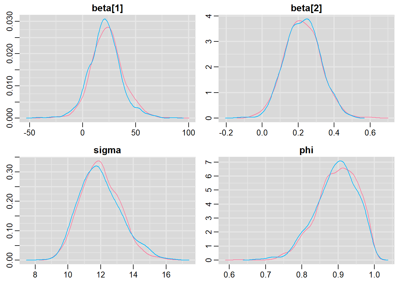

> traplot(mcmc, parms = c("beta", "sigma", "phi"))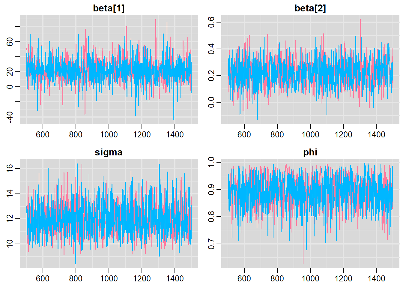

> #Raftery diagnostic
> raftery.diag(mcmc)
[[1]]

Quantile (q) = 0.025
Accuracy (r) = +/- 0.005
Probability (s) = 0.95 

You need a sample size of at least 3746 with these values of q, r and s

[[2]]

Quantile (q) = 0.025
Accuracy (r) = +/- 0.005
Probability (s) = 0.95 

You need a sample size of at least 3746 with these values of q, r and s

> #Autocorrelation diagnostic
> autocorr.diag(mcmc)
            beta[1]      beta[2]        sigma           phi        lp__
Lag 0   1.000000000  1.000000000  1.000000000  1.000000e+00  1.00000000
Lag 1   0.152178661  0.181655778  0.062722850  9.682982e-02  0.45706648
Lag 5  -0.001128217  0.001348094  0.007963621  1.390360e-02  0.04092522
Lag 10  0.026325475 -0.010276373 -0.048228887 -1.750250e-02 -0.00619533
Lag 50  0.004569914 -0.033128415 -0.023918937  3.767909e-05 -0.01373323

> stan_ac(data.temporalCor2.rstan)

> stan_rhat(data.temporalCor2.rstan)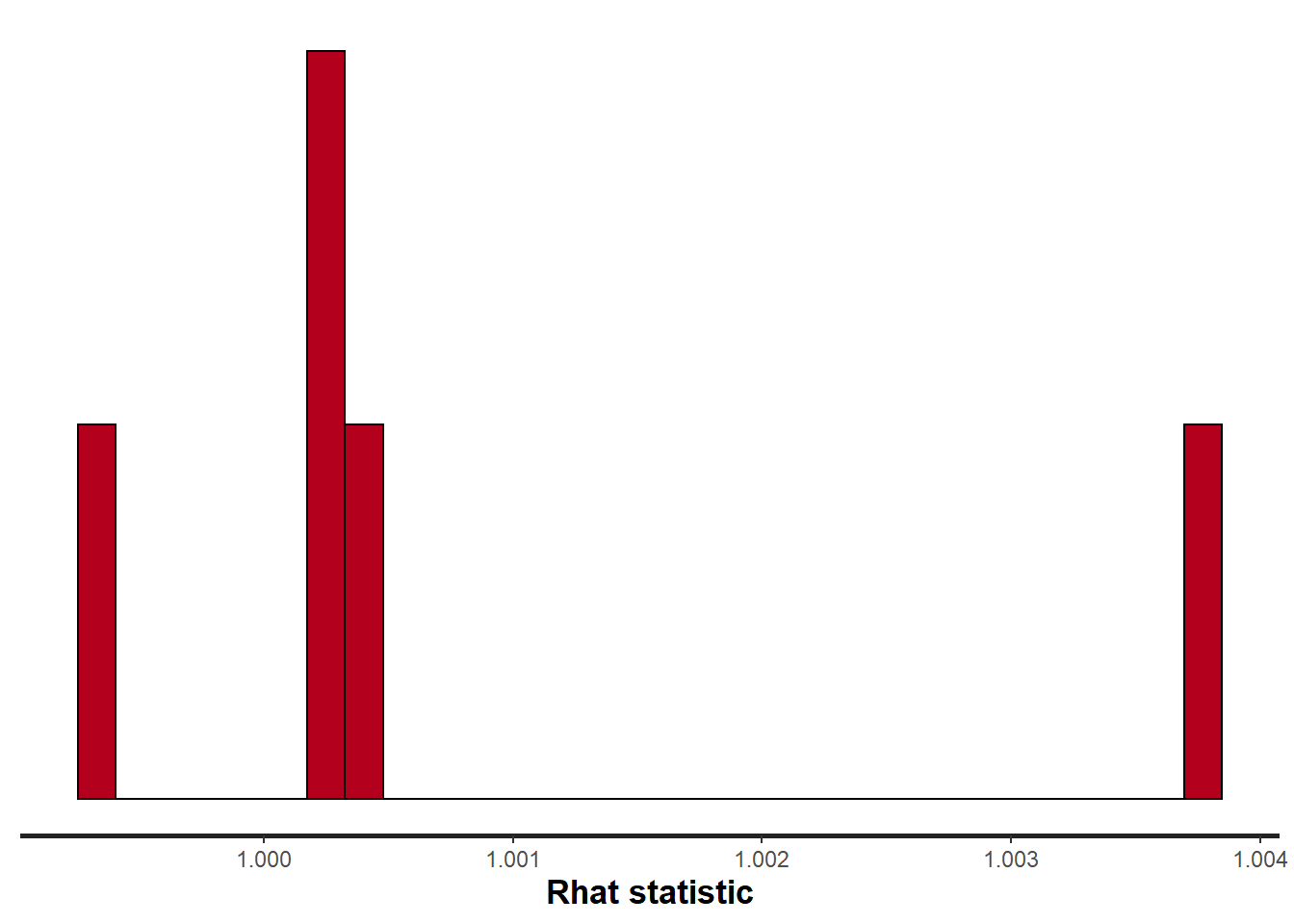

> stan_ess(data.temporalCor2.rstan)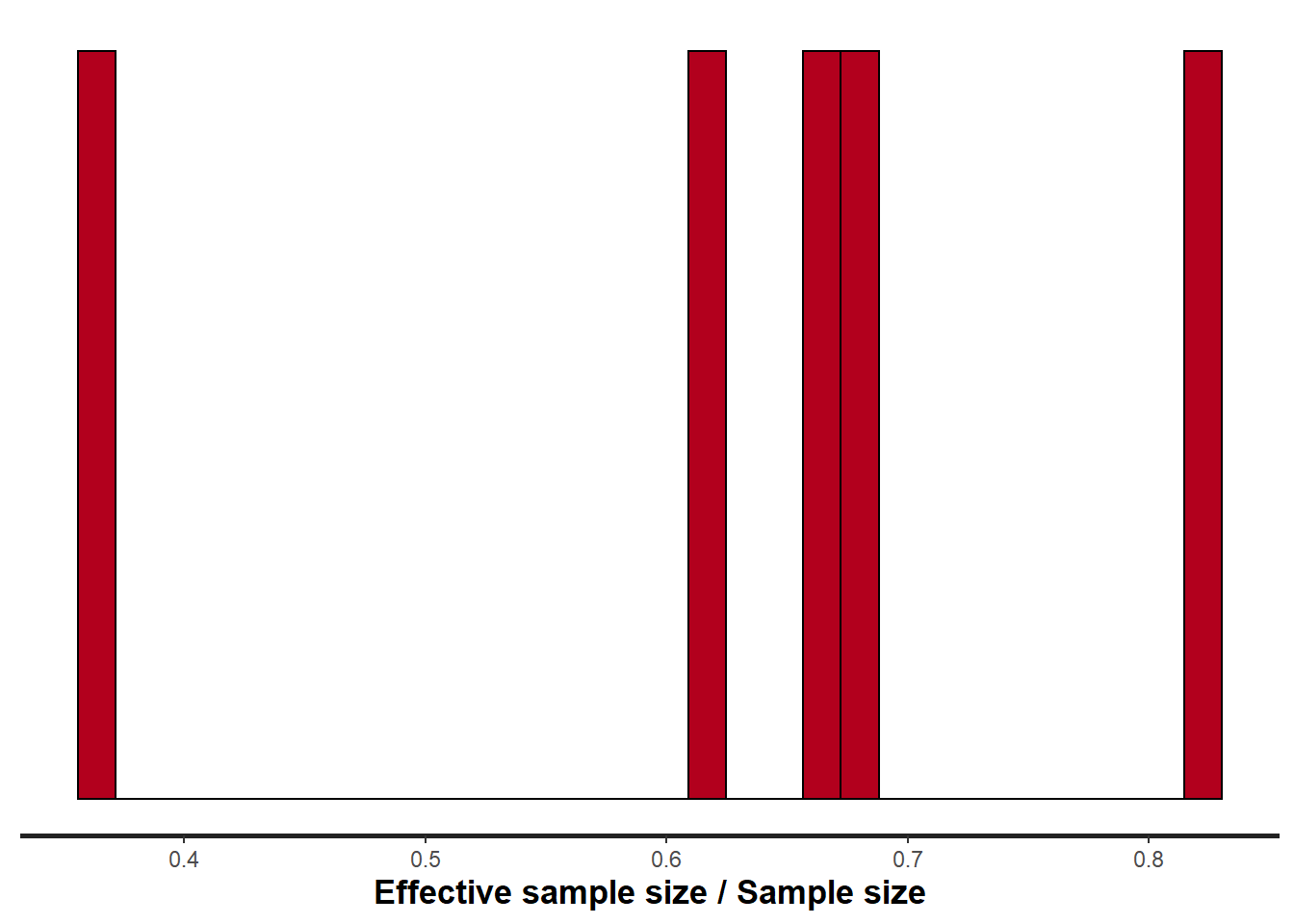

All diagnostics seem fine.

Model validation

\[ Res_i = Y_i - \mu_i\]

\[ Res_{i+1} = Res_{i+1} - \rho Res_i\]

\[ Res_i = \frac{Res_i}{\sigma} \]

> mcmc = as.matrix(data.temporalCor2.rstan)
> wch = grep("beta", colnames(mcmc))
> # generate a model matrix
> newdata = data.frame(x = data.temporalCor$x)
> Xmat = model.matrix(~x, newdata)
> ## get median parameter estimates
> coefs = mcmc[, wch]
> fit = coefs %*% t(Xmat)
> resid = -1 * sweep(fit, 2, data.temporalCor$y, "-")
> n = ncol(resid)
> resid[, -1] = resid[, -1] - (resid[, -n] * mcmc[, "phi"])
> resid = apply(resid, 2, median)/median(mcmc[, "sigma"])
> fit = apply(fit, 2, median)
> 
> ggplot() + geom_point(data = NULL, aes(y = resid, x = fit)) + theme_classic()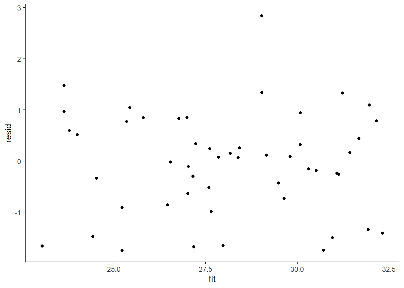

> 
> ggplot() + geom_point(data = NULL, aes(y = resid, x = data.temporalCor$x)) + theme_classic()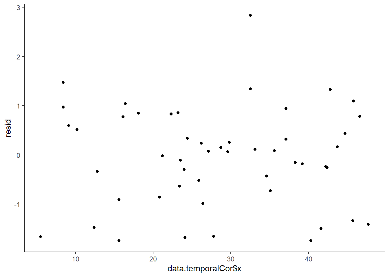

> 
> ggplot(data = NULL, aes(y = resid, x = data.temporalCor$year)) +
+     geom_point() + geom_line() + geom_hline(yintercept = 0, linetype = "dashed") + theme_classic()

> 
> plot(acf(resid, lag = 40))

> 
> fit = coefs %*% t(Xmat)
> ## draw samples from this model
> yRep = sapply(1:nrow(mcmc), function(i) rnorm(nrow(data.temporalCor),
+     fit[i, ], mcmc[i, "sigma"]))
> ggplot() + geom_density(data = NULL, aes(x = as.vector(yRep),
+     fill = "Model"), alpha = 0.5) + geom_density(data = data.temporalCor,
+     aes(x = y, fill = "Obs"), alpha = 0.5) + theme_classic()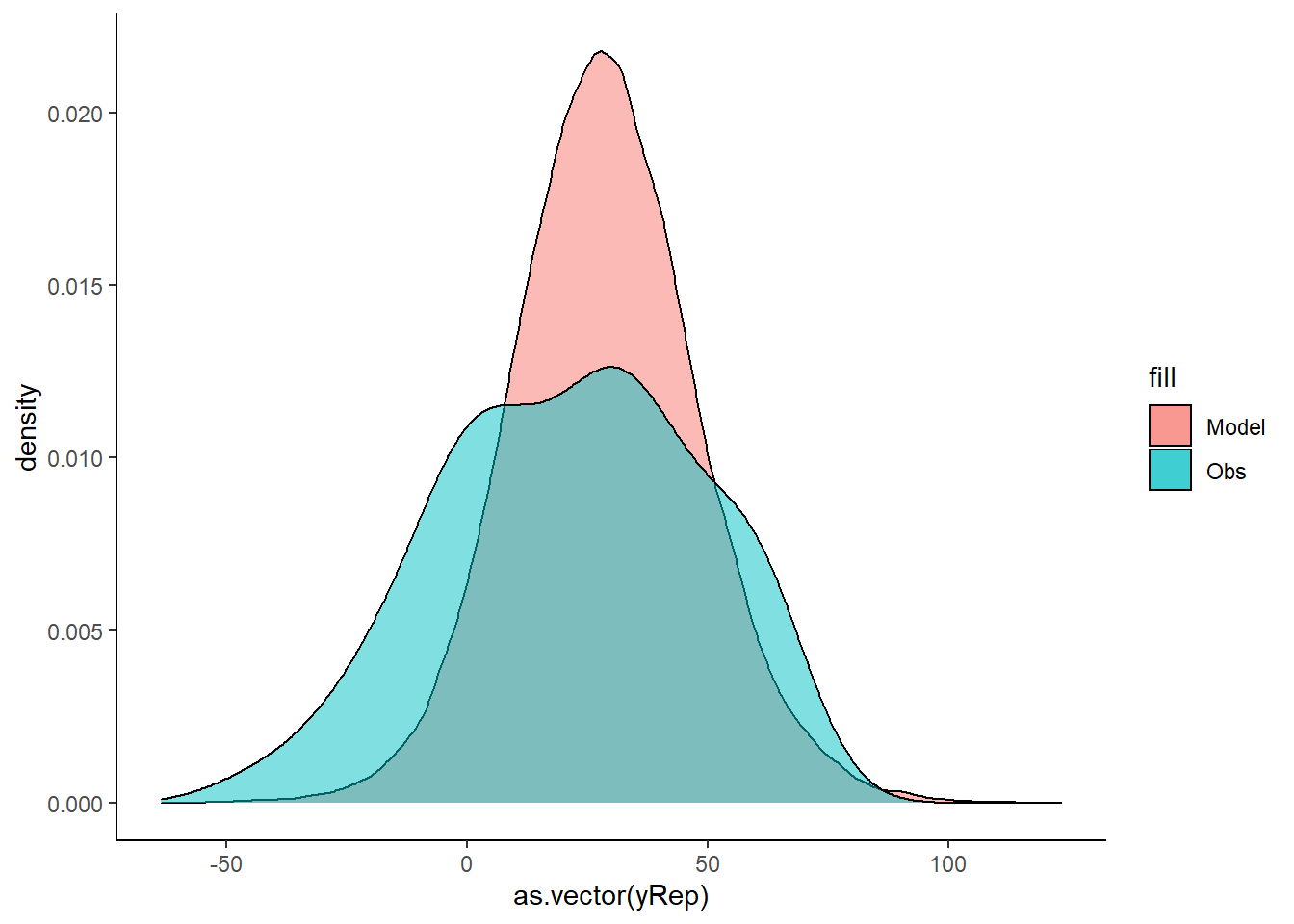

No obvious autocorrelation or other issues with residuals remaining.

Parameter estimates

Explore parameter estimates.

> tidyMCMC(data.temporalCor2.rstan, par = c("beta", "phi", "sigma"),
+     conf.int = TRUE, conf.method = "HPDinterval", rhat = TRUE,
+     ess = TRUE)
# A tibble: 4 x 7
  term    estimate std.error conf.low conf.high  rhat   ess
  <chr>      <dbl>     <dbl>    <dbl>     <dbl> <dbl> <int>
1 beta[1]   21.9     15.1     -7.40      53.6   1.00   1321
2 beta[2]    0.224    0.0974   0.0501     0.426 1.00   1220
3 phi        0.900    0.0560   0.789      0.989 1.00   1355
4 sigma     11.9      1.23     9.75      14.5   0.999  1659

References

Gelman, Andrew, Daniel Lee, and Jiqiang Guo. 2015. “Stan: A Probabilistic Programming Language for Bayesian Inference and Optimization.” Journal of Educational and Behavioral Statistics 40 (5): 530–43.

Stan Development Team. 2018. “RStan: The R Interface to Stan.” http://mc-stan.org/.

tutorials Stan autocorrelation

Temporal Autocorrelation (Stan)

Overview

Introduction

First order autocorrelation

Incorporating lagged residuals

Model fitting

MCMC diagnostics

Model validation

Parameter estimates

Incorporating AR1 residual autocorrelation structure

Model fitting

MCMC diagnostics

Model validation

Parameter estimates

References

Assistant Professor in Statistics