Super basic introduction to JAGS
The focus of this simple tutorial is to provide a brief introduction and overview about how to fit Bayesian models using JAGS via R.
Prerequisites:
- The latest version of
R, which can be downloaded and installed for Windows, Mac or Linux OS from the CRAN website - I also strongly recommend to download and install Rstudio, an integrated development environment which provides an “user-friendly” interaction with
R(e.g. many drop-down menus, tabs, customisation options)
Preliminaries
What is JAGS?
JAGS or Just Another Gibbs Sampler is a program for analysis of Bayesian models using Markov Chain Monte Carlo (MCMC) methods (Plummer (2004)). JAGS is a free software based on the Bayesian inference Using Gibbs Sampling (informally BUGS) language at the base of WinBUGS/OpenBUGS but, unlike these programs, it is written in C++ and is platform independent. The latest version of JAGS can be dowloaded from Martyn Plummer’s repository and is available for different OS. There are different R packages which function as frontends for JAGS. These packages make it easy to process the output of Bayesian models and present it in publication-ready form. In this brief introduction, I will specifically focus on the R2jags package (Su et al. (2015)) and show how to fit JAGS models using this package.
Installing JAGS and R2jags
Install the latest version of JAGS for your OS. Next, install the package R2jags from within R or Rstudio, via the package installer or by typing in the command line
> install.packages("R2jags", dependencies = TRUE)The dependencies = TRUE option will automatically install all the packages on which the functions in the R2jags package rely.
Basic model
Simulate data
For an example dataset, I simulate my own data in R. I create a continuous outcome variable \(y\) as a function of one predictor \(x\) and a disturbance term \(\epsilon\). I simulate a dataset with 100 observations. Create the error term, the predictor and the outcome using a linear form with an intercept \(\beta_0\) and slope \(\beta_1\) coefficients, i.e.
\[y = \beta_0 + \beta_1 x + \epsilon \]
The R commands which I use to simulate the data are the following:
> n.sim=100; set.seed(123)
> x=rnorm(n.sim, mean = 5, sd = 2)
> epsilon=rnorm(n.sim, mean = 0, sd = 1)
> beta0=1.5
> beta1=1.2
> y=beta0 + beta1 * x + epsilon
Then, I define all the data for JAGS in a list object
> datalist=list("y","x","n.sim")Model file
Now, I write the model for JAGS and save it as a text file named "basic.mod.txt" in the current working directory
> basic.mod= "
+ model {
+ #model
+  for(i in 1:n.sim){
+   y[i] ~ dnorm(mu[i], tau)
+   mu[i] = beta0 + beta1 * x[i]
+  }
+ #priors
+ beta0 ~ dnorm(0, 0.01)
+ beta1 ~ dnorm(0, 0.01)
+ tau ~ dgamma(0.01,0.01)
+ }
+ "
The part of the model inside the for loop denotes the likelihood, which is evaluated for each individual in the sample using a Normal distribution parameterised by some mean mu and precision tau (where, precision = 1/variance). The covariate x is included at the mean level using a linear regression, which is indexed by the intercept beta0 and slope beta1 terms. The second part defines the prior distributions for all parameters of the model, namely the regression coefficients and the precision. Weakly informative priors are used since I assume that I do not have any prior knowledge about these parameters.
To write and save the model as the text file “basic.mod.txt” in the current working directory, I use the writeLines function
> writeLines(basic.mod, "basic.mod.txt")Pre-processing
Define the parameters whose posterior distribtuions we are interested in summarising later and set up the initial values for the MCMC sampler in JAGS
> params=c("beta0","beta1")
> inits=function(){list("beta0"=rnorm(1), "beta1"=rnorm(1))}
The function creates a list that contains one element for each parameter, which gets assigned a random draw from a normal distribution as a strating value for each chain in the model. For simple models like this, it is generally easy to define the intial values for all parameters. However, for more complex models, this may not be immediate and a lot of trial and error may be required. However, JAGS can automatically select the initial values for all parameters in an efficient way even for relatively complex models. This can be achieved by setting inits=NULL, which is then passed to the jags function in R2jags.
Before using R2jags for the first time, you need to load the package, and you may want to set a random seed number for making your estimates replicable
> library(R2jags)
> set.seed(123)
Fit the model
Now, we can fit the model in JAGS using the jags function in the R2jags package and save it in the object basic.mod
> basic.mod=jags(data = datalist, inits = inits,
+   parameters.to.save = params, n.chains = 2, n.iter = 2000,
+   n.burnin = 1000, model.file = "basic.mod.txt")
Compiling model graph
   Resolving undeclared variables
   Allocating nodes
Graph information:
   Observed stochastic nodes: 100
   Unobserved stochastic nodes: 3
   Total graph size: 406

Initializing model
While the model is running, the function prints out some information related to the Bayesian graph (corresponding to the specification used for the model) underneath JAGS, such as number of observed and unobserved nodes and graph size.
Post-processing
Once the model has finished running, a summary of the posteiror estimates and convergence diagnostics for all parameters specified can be seen by typing print(basic.mod) or, alternatively,
> print(basic.mod$BUGSoutput$summary) mean sd 2.5% 25% 50% 75% 97.5% Rhat n.eff
beta0 1.5 0.294 0.95 1.3 1.5 1.7 2.1 1 2000
beta1 1.2 0.054 1.07 1.1 1.2 1.2 1.3 1 2000
deviance 278.8 2.475 276.03 277.1 278.2 279.9 285.1 1 2000The posterior distribution of each parameter is summarised in terms of:
- The mean, sd and some percentiles
- Potential scale reduction factor
Rhatand effective sample sizen.eff(Gelman et al. (2013)). The first is a measure to assess issues in convergence of the MCMC algorithm (typically a value below \(1.05\) for all parameters is considered ok). The second is a measure which assesses the adequacy of the posterior sample (typically values close to the total number of iterations are desirable for all parameters).
The deviance is a goodness of fit statistic and is used in the construction of the “Deviance Information Criterion” or DIC (Spiegelhalter et al. (2014)), which is a relative measure of model comparison. The DIC of the model can be accessed by typing
> basic.mod$BUGSoutput$DIC
[1] 282
Diagnostics
More diagnostics are available when we convert the model output into an MCMC object using the command
> basic.mod.mcmc=as.mcmc(basic.mod)Different packages are available to perform diagnostic checks for Bayesian models. Here, I install and load the mcmcplots package (Curtis (2015)) to obtain graphical diagnostics and results.
> install.packages("mcmcplots")
> library(mcmcplots)
For example, density and trace plots can be obtained by typing
> denplot(basic.mod.mcmc, parms = c("beta0","beta1"))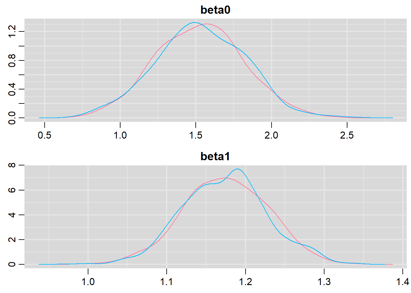
> traplot(basic.mod.mcmc, parms = c("beta0","beta1"))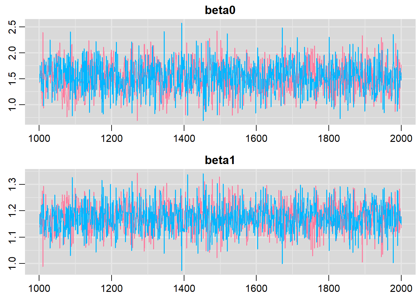
Both types of graphs suggest that there are not issues in the convergence of the algorithm (smooth normal densities and hairy caterpillar graphs for both MCMC chains).
Conclusions
This tutorial was simply a brief introduction on how simple linear regression models can be fitted using the Bayesian software JAGS via the R2jags package. Although this may seem a complex procedure compared with simply fitting a linear model under the frequentist framework, however, the real advantages of Bayesian methods become evident when the complexity of the analysis is increased (which is often the case in real applications). Indeed, the flexibility in Bayesian modelling allows to account for increasingly complex models in a relatively easy way. In addition, Bayesian methods are ideal when the interest is in taking into account the potential impact that different sources of uncertainty may have on the final results, as they allow the natural propagation of uncertainty throughout each quantity in the model.