Data generation

We will start by generating a random data set. Note, I am creating two versions of the predictor variable (a numeric version and a factorial version).

> set.seed(123)
> nA <- 60  #sample size from Population A
> nB <- 40  #sample size from Population B
> muA <- 105  #population mean of Population A
> muB <- 77.5  #population mean of Population B
> sigma <- 3  #standard deviation of both populations (equally varied)
> yA <- rnorm(nA, muA, sigma)  #Population A sample
> yB <- rnorm(nB, muB, sigma)  #Population B sample
> y <- c(yA, yB)
> x <- factor(rep(c("A", "B"), c(nA, nB)))  #categorical listing of the populations
> xn <- as.numeric(x)  #numerical version of the population category for means parameterization. # Should not start at 0.
> data <- data.frame(y, x, xn)  # dataset

Let inspect the first few rows of the dataset using the command head

> head(data)
         y x xn
1 103.3186 A  1
2 104.3095 A  1
3 109.6761 A  1
4 105.2115 A  1
5 105.3879 A  1
6 110.1452 A  1

We can also perform some exploratory data analysis - in this case, a boxplot of the response for each level of the predictor.

> boxplot(y ~ x, data)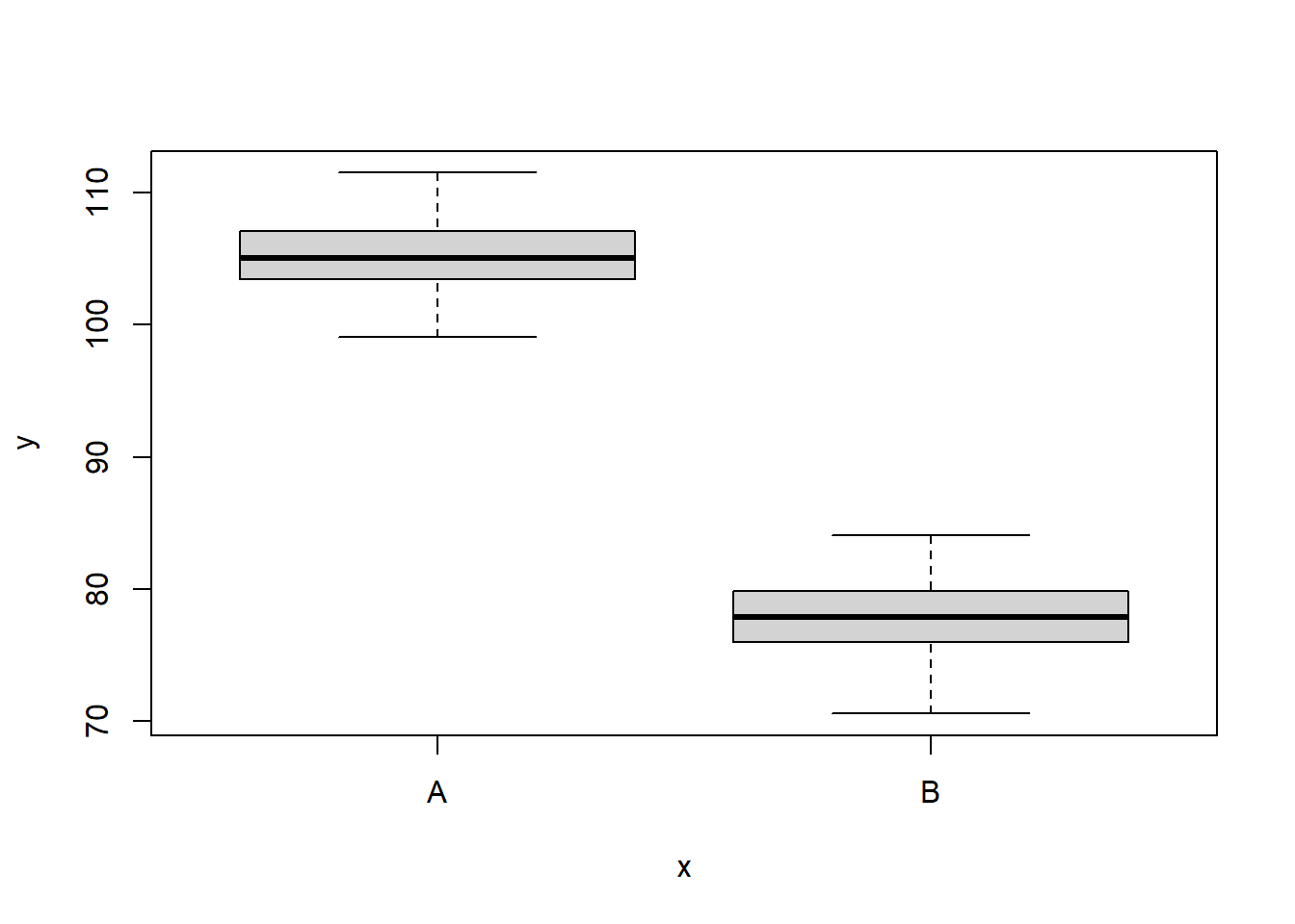

The One Sample t-test

A t-test is essentially just a simple regression model in which the categorical predictor is represented by a binary variable in which one level is coded as \(0\) and the other \(1\). For the model itself, the observed response \(y_i\) are assumed to be drawn from a normal distribution with a given mean \(\mu\) and standard deviation \(\sigma\). The expected values are themselves determined by the linear predictor \(\mu_i=\beta_0+\beta_1x_i\), where \(\beta_0\) represents the mean of the first treatment group and \(\beta_1\) represents the difference between the mean of the first group and the mean of the second group (the effect of interest).

MCMC sampling requires priors on all parameters. We will employ weakly informative priors. Specifying “uninformative” priors is always a bit of a balancing act. If the priors are too vague (wide) the MCMC sampler can wander off into nonscence areas of likelihood rather than concentrate around areas of highest likelihood (desired when wanting the outcomes to be largely driven by the data). On the other hand, if the priors are too strong, they may have an influence on the parameters. In such a simple model, this balance is very forgiving - it is for more complex models that prior choice becomes more important. For this simple model, we will go with zero-centered Gaussian (normal) priors with relatively large standard deviations (\(1000\)) for both the intercept and the treatment effect and a wide half-cauchy (scale=\(25\)) for the standard deviation (Gelman and others (2006)).

\[y_i \sim \text{Normal}(\mu_i, \sigma), \]

where \(\mu_i=\beta_0+\beta_1x_i\).

Priors are defined as:

\[ \beta_j \sim \text{Normal}(0,1000), \;\;\; \text{and} \;\;\; \sigma \sim \text{Cauchy}(0,25), \]

for \(j=0,1\).

> modelString = "  
+  model {
+   #Likelihood
+   for (i in 1:n) {
+     y[i]~dnorm(mu[i],tau)
+     mu[i] <- beta0+beta[x[i]]
+   }
+  
+   #Priors
+   beta0 ~ dnorm(0,1.0E-06)
+   beta[1] <- 0
+   beta[2] ~ dnorm(0,1.0E-06)
+   tau ~ dgamma(0.1,0.1)
+   sigma<-1/sqrt(tau)
+ 
+   #Other Derived parameters 
+   # Group means (note, beta is a vector)
+   Group.means <-beta0+beta  
+  }
+  "
> ## write the model to a text file
> writeLines(modelString, con = "ttestModel.txt")

> modelString.means = "  
+   model {
+    #Likelihood 
+    for (i in 1:n) {
+      y[i]~dnorm(mu[i],tau)
+      mu[i] <- beta[x[i]]
+    }
+  
+    #Priors
+    for (j in min(x):max(x)) {
+      beta[j] ~ dnorm(0,0.001)
+    }
+  
+    tau~dgamma(0.1,0.1)
+    sigma<-1/sqrt(tau)
+  
+    #Other Derived parameters 
+    effect <-beta[2]-beta[1]
+  }
+  "
> 
> ## write the model to a text file
> writeLines(modelString.means, con = "ttestModelMeans.txt")

> data.list <- with(data, list(y = y, x = xn, n = nrow(data)))
> data.list.means <- with(data, list(y = y, x = xn, n = nrow(data)))

> inits <- list(beta0 = mean(data$y), beta = c(NA, diff(tapply(data$y,
+     data$x, mean))), sigma = sd(data$y/2))
> inits.means <- list(beta = tapply(data$y, data$x, mean), sigma = sd(data$y/2))

> params <- c("beta0", "beta", "sigma", "Group.means")
> params.means <- c("beta", "effect", "sigma")

> adaptSteps = 1000  # the number of steps over which to establish a good stepping distance
> burnInSteps = 2000  # the number of initial samples to discard
> nChains = 2  # the number of independed sampling chains to perform 
> numSavedSteps = 50000  # the total number of samples to store
> thinSteps = 1  # the thinning rate
> nIter = ceiling((numSavedSteps * thinSteps)/nChains)

> library(R2jags)

> data.r2jags <- jags(data=data.list,
+ inits=NULL, #or inits=list(inits,inits) # since there are two chains
+ parameters.to.save=params,
+ model.file="ttestModel.txt",
+ n.chains=nChains,
+ n.iter=nIter,
+ n.burnin=burnInSteps,
+ n.thin=thinSteps)
Compiling model graph
   Resolving undeclared variables
   Allocating nodes
Graph information:
   Observed stochastic nodes: 100
   Unobserved stochastic nodes: 3
   Total graph size: 214

Initializing model
> 
> #print results
> print(data.r2jags)
Inference for Bugs model at "ttestModel.txt", fit using jags,
 2 chains, each with 25000 iterations (first 2000 discarded)
 n.sims = 46000 iterations saved
               mu.vect sd.vect    2.5%     25%     50%     75%   97.5%  Rhat
Group.means[1] 105.200   0.357 104.497 104.959 105.201 105.441 105.900 1.001
Group.means[2]  77.882   0.438  77.018  77.589  77.882  78.174  78.746 1.001
beta[1]          0.000   0.000   0.000   0.000   0.000   0.000   0.000 1.000
beta[2]        -27.318   0.563 -28.426 -27.696 -27.315 -26.943 -26.212 1.001
beta0          105.200   0.357 104.497 104.959 105.201 105.441 105.900 1.001
sigma            2.771   0.202   2.408   2.630   2.759   2.900   3.198 1.001
deviance       487.192   2.485 484.376 485.370 486.547 488.331 493.506 1.001
               n.eff
Group.means[1] 46000
Group.means[2] 15000
beta[1]            1
beta[2]        35000
beta0          46000
sigma          46000
deviance       46000

For each parameter, n.eff is a crude measure of effective sample size,
and Rhat is the potential scale reduction factor (at convergence, Rhat=1).

DIC info (using the rule, pD = var(deviance)/2)
pD = 3.1 and DIC = 490.3
DIC is an estimate of expected predictive error (lower deviance is better).

> data.r2jags.means <- jags(data=data.list.means,
+ inits=NULL, #or inits=list(inits.means,inits.means) # since there are two chains
+ parameters.to.save=params.means,
+ model.file="ttestModelMeans.txt",
+ n.chains=nChains,
+ n.iter=nIter,
+ n.burnin=burnInSteps,
+ n.thin=thinSteps)
Compiling model graph
   Resolving undeclared variables
   Allocating nodes
Graph information:
   Observed stochastic nodes: 100
   Unobserved stochastic nodes: 3
   Total graph size: 211

Initializing model
> 
> #print results
> print(data.r2jags.means)
Inference for Bugs model at "ttestModelMeans.txt", fit using jags,
 2 chains, each with 25000 iterations (first 2000 discarded)
 n.sims = 46000 iterations saved
         mu.vect sd.vect    2.5%     25%     50%     75%   97.5%  Rhat n.eff
beta[1]  105.184   0.357 104.481 104.947 105.184 105.423 105.884 1.001 46000
beta[2]   77.867   0.439  77.001  77.575  77.866  78.160  78.736 1.001 39000
effect   -27.317   0.566 -28.433 -27.696 -27.317 -26.940 -26.197 1.001 46000
sigma      2.768   0.201   2.408   2.626   2.755   2.897   3.192 1.001 34000
deviance 487.195   2.498 484.360 485.377 486.540 488.323 493.721 1.001 46000

For each parameter, n.eff is a crude measure of effective sample size,
and Rhat is the potential scale reduction factor (at convergence, Rhat=1).

DIC info (using the rule, pD = var(deviance)/2)
pD = 3.1 and DIC = 490.3
DIC is an estimate of expected predictive error (lower deviance is better).

MCMC diagnostics

In addition to the regular model diagnostic checks (such as residual plots), for Bayesian analyses, it is necessary to explore the characteristics of the MCMC chains and the sampler in general. Recall that the purpose of MCMC sampling is to replicate the posterior distribution of the model likelihood and priors by drawing a known number of samples from this posterior (thereby formulating a probability distribution). This is only reliable if the MCMC samples accurately reflect the posterior. Unfortunately, since we only know the posterior in the most trivial of circumstances, it is necessary to rely on indirect measures of how accurately the MCMC samples are likely to reflect the likelihood. I will briefly outline the most important diagnostics.

• Traceplots for each parameter illustrate the MCMC sample values after each successive iteration along the chain. Bad chain mixing (characterised by any sort of pattern) suggests that the MCMC sampling chains may not have completely traversed all features of the posterior distribution and that more iterations are required to ensure the distribution has been accurately represented.

• Autocorrelation plot for each parameter illustrate the degree of correlation between MCMC samples separated by different lags. For example, a lag of \(0\) represents the degree of correlation between each MCMC sample and itself (obviously this will be a correlation of \(1\)). A lag of \(1\) represents the degree of correlation between each MCMC sample and the next sample along the chain and so on. In order to be able to generate unbiased estimates of parameters, the MCMC samples should be independent (uncorrelated).

• Potential scale reduction factor (Rhat) statistic for each parameter provides a measure of sampling efficiency/effectiveness. Ideally, all values should be less than \(1.05\). If there are values of \(1.05\) or greater it suggests that the sampler was not very efficient or effective. Not only does this mean that the sampler was potentially slower than it could have been but, more importantly, it could indicate that the sampler spent time sampling in a region of the likelihood that is less informative. Such a situation can arise from either a misspecified model or overly vague priors that permit sampling in otherwise nonscence parameter space.

Prior to examining the summaries, we should have explored the convergence diagnostics. We use the package mcmcplots to obtain density and trace plots for the effects model as an example.

> library(mcmcplots)
> denplot(data.r2jags, parms = c("beta0","beta[2]","sigma"))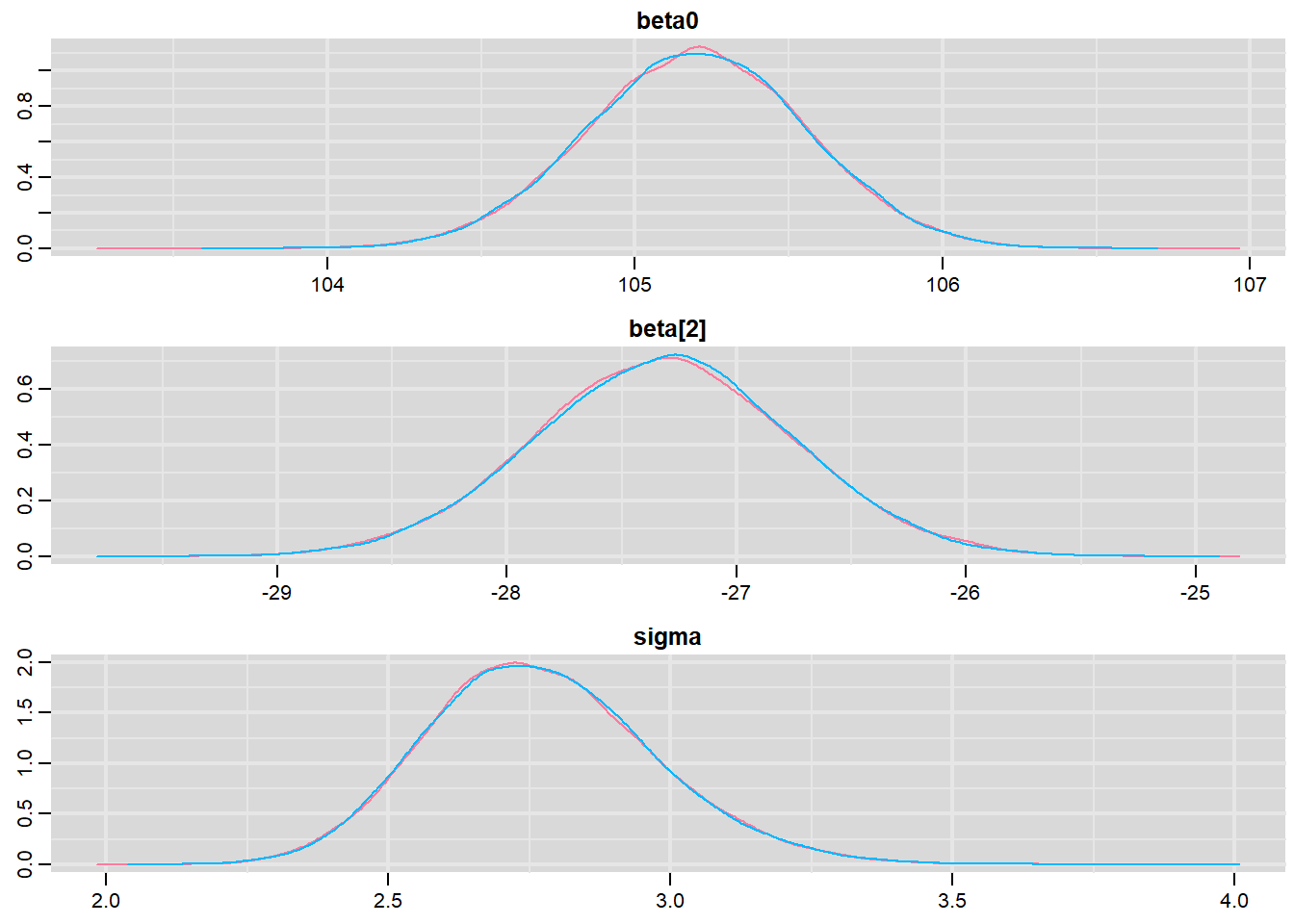

> traplot(data.r2jags, parms = c("beta0","beta[2]","sigma"))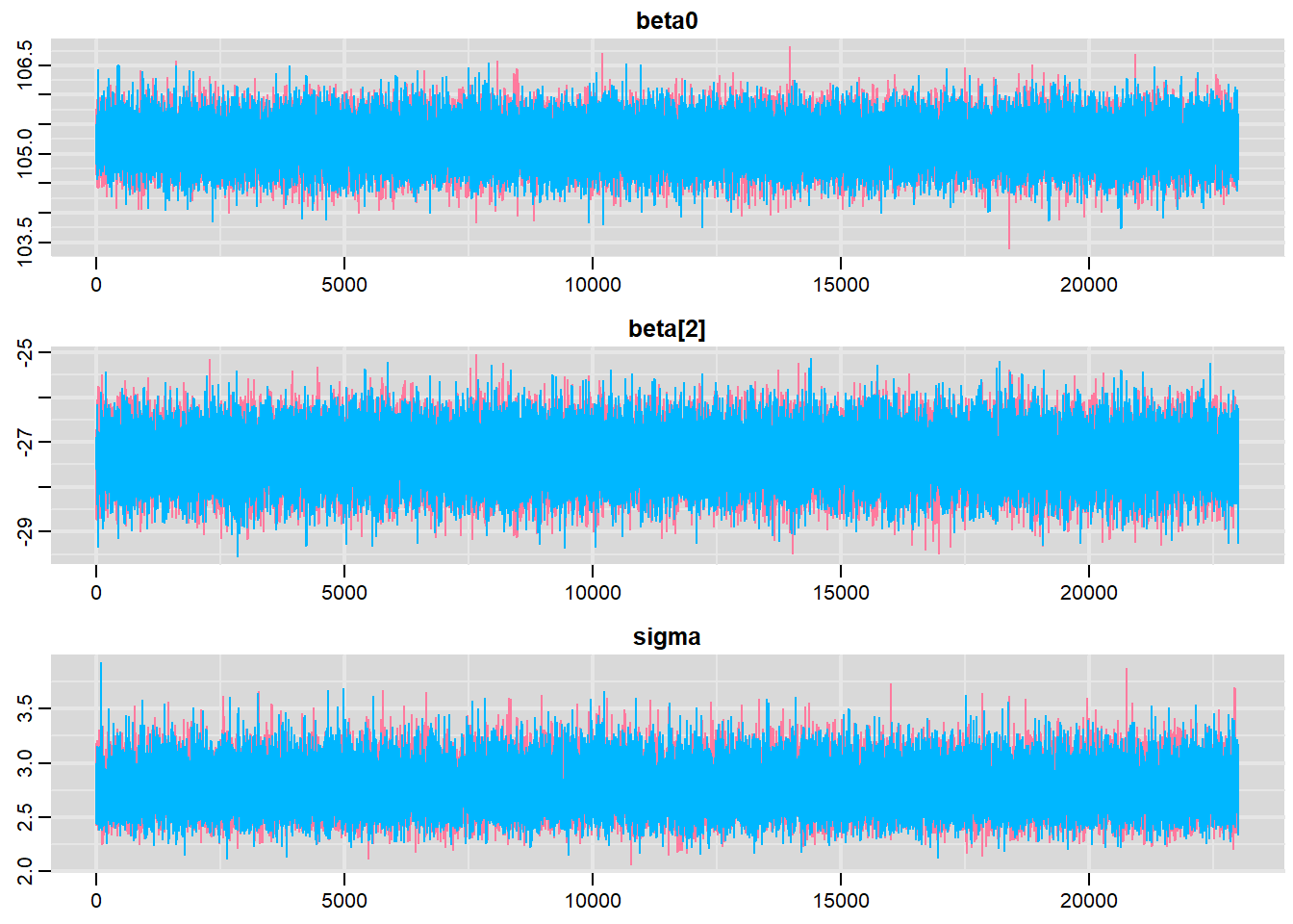

These plots show no evidence that the chains have not reasonably traversed the entire multidimensional parameter space.

Model validation

Model validation involves exploring the model diagnostics and fit to ensure that the model is broadly appropriate for the data. As such, exploration of the residuals should be routine. Ideally, a good model should also be able to predict the data used to fit the model.

Residuals are not computed directly within R2jags. However, we can calculate them manually form the posteriors and plot them using the package ggplot2.

> library(ggplot2)
> mcmc = data.r2jags$BUGSoutput$sims.matrix[, c("beta0", "beta[2]")]
> # generate a model matrix
> newdata = data.frame(x = data$x)
> Xmat = model.matrix(~x, newdata)
> ## get median parameter estimates
> coefs = apply(mcmc, 2, median)
> fit = as.vector(coefs %*% t(Xmat))
> resid = data$y - fit
> ggplot() + geom_point(data = NULL, aes(y = resid, x = fit))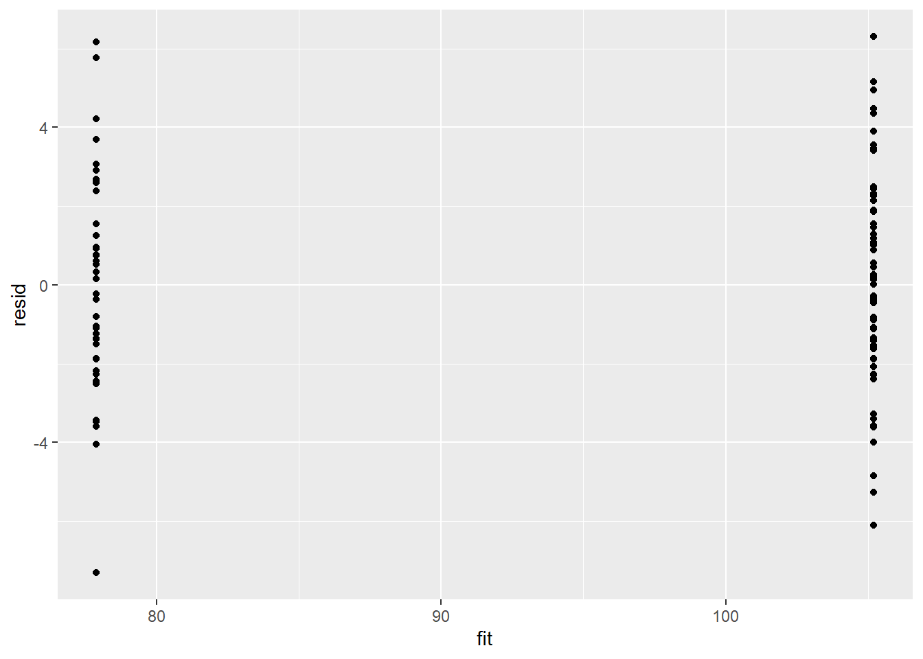

There is no evidence that the mcmc chain did not converge on a stable posterior distribution. We are now in a position to examine the summaries of the parameters.

Parameter estimates

Although all parameters in a Bayesian analysis are considered random and are considered a distribution, rarely would it be useful to present tables of all the samples from each distribution. On the other hand, plots of the posterior distributions have some use. Nevertheless, most workers prefer to present simple statistical summaries of the posteriors. Popular choices include the median (or mean) and \(95\)% credibility intervals.

> library(broom)
> library(broom.mixed)
> tidyMCMC(as.mcmc(data.r2jags), conf.int = TRUE, conf.method = "HPDinterval")
# A tibble: 6 x 5
  term           estimate std.error conf.low conf.high
  <chr>             <dbl>     <dbl>    <dbl>     <dbl>
1 Group.means[1]   105.       0.357   105.      106.  
2 Group.means[2]    77.9      0.438    77.0      78.7 
3 beta[1]            0        0         0         0   
4 beta[2]          -27.3      0.563   -28.4     -26.2 
5 beta0            105.       0.357   105.      106.  
6 sigma              2.76     0.202     2.39      3.17

The Group A is typically \(27.3\) units greater than Group B. The \(95\)% confidence interval for the difference between Group A and B does not overlap with \(0\) implying a significant difference between the two groups.

Graphical summaries

A nice graphic is often a great accompaniment to a statistical analysis. Although there are no fixed assumptions associated with graphing (in contrast to statistical analyses), we often want the graphical summaries to reflect the associated statistical analyses. After all, the sample is just one perspective on the population(s). What we are more interested in is being able to estimate and depict likely population parameters/trends. Thus, whilst we could easily provide a plot displaying the raw data along with simple measures of location and spread, arguably, we should use estimates that reflect the fitted model. In this case, it would be appropriate to plot the credibility interval associated with each group. We do this by loading functions in the package dplyr.

> library(dplyr)
> mcmc = data.r2jags$BUGSoutput$sims.matrix
> ## Calculate the fitted values
> newdata = data.frame(x = levels(data$x))
> Xmat = model.matrix(~x, newdata)
> coefs = mcmc[, c("beta0", "beta[2]")]
> fit = coefs %*% t(Xmat)
> newdata = newdata %>% cbind(tidyMCMC(fit, conf.int = TRUE, conf.method = "HPDinterval"))
> 
> ggplot(newdata, aes(y = estimate, x = x)) + geom_pointrange(aes(ymin = conf.low,
+     ymax = conf.high)) + scale_y_continuous("Y") + scale_x_discrete("X") +
+     theme_classic()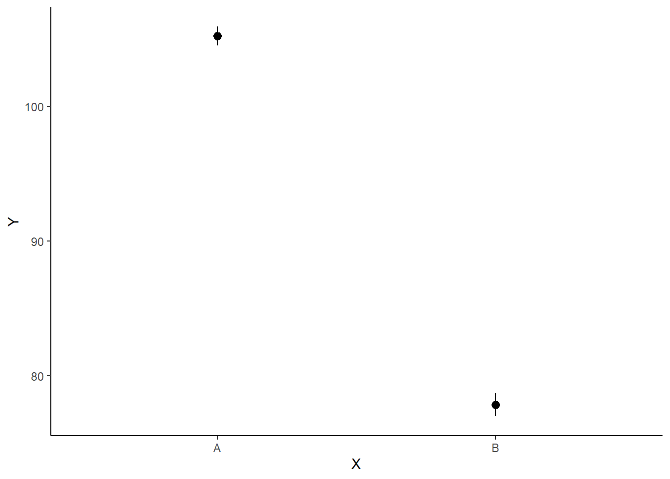

If you wanted to represent sample data on the figure in such a simple example (single predictor) we could simply over- (or under-) lay the raw data.

> ggplot(newdata, aes(y = estimate, x = x)) + geom_point(data = data, aes(y = y,
+     x = x), color = "gray") + geom_pointrange(aes(ymin = conf.low, ymax = conf.high)) +
+     scale_y_continuous("Y") + scale_x_discrete("X") + theme_classic()

A more general solution would be to add the partial residuals to the figure. Partial residuals are the fitted values plus the residuals. In this simple case, that equates to exactly the same as the raw observations since \(\text{resid}=\text{obs}−\text{fitted}\) and the fitted values depend only on the single predictor we are interested in.

> ## Calculate partial residuals fitted values
> fdata = rdata = data
> fMat = rMat = model.matrix(~x, fdata)
> fit = as.vector(apply(coefs, 2, median) %*% t(fMat))
> resid = as.vector(data$y - apply(coefs, 2, median) %*% t(rMat))
> rdata = rdata %>% mutate(partial.resid = resid + fit)
> ggplot(newdata, aes(y = estimate, x = x)) + geom_point(data = rdata, aes(y = partial.resid),
+     color = "gray") + geom_pointrange(aes(ymin = conf.low, ymax = conf.high)) +
+     scale_y_continuous("Y") + scale_x_discrete("X") + theme_classic()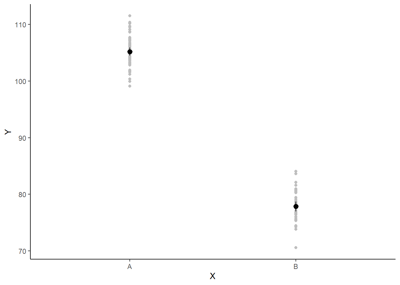

Effect sizes

In addition to deriving the distribution means for the second group, we could make use of the Bayesian framework to derive the distribution of the effect size. There are multiple ways of calculating an effect size, but the most common are:

• Raw effect size - the difference between two groups (as already calculated)

• Cohen’s D - the effect size standardised by division with the pooled standard deviation

• Percent - the effect size expressed as a percent of the reference group mean

Calculating the percent effect size involves division by an estimate of \(\beta_0\). The very first sample collected of each parameter (including \(\beta_0\)) is based on the initial values supplied. If inits=NULL the jags function appears to generate initial values from the priors. Recall that in the previous model definition, \(\beta_0\) was deemed to be distributed as a normal distribution with a mean of \(0\). Hence, \(\beta_0\) would initially be assigned a value of \(0\). Division by zero is of course illegal and thus an error would be thrown. There are two ways to overcome this:

• Modify the prior such that it has a mean close to zero (and thus the first \(\beta_0\) sample is not zero), yet not actually zero (such as \(0.0001\)). This is the method used here.

• Define initial values that are based on the observed data (and not zero).

> paramsv2 <- c("beta0", "beta", "sigma", "Group.means", "cohenD", "ES", "p10")
> data.r2jagsv2 <- jags(data=data.list,
+ inits=NULL, #or inits=list(inits,inits) # since there are two chains
+ parameters.to.save=paramsv2,
+ model.file="ttestModelv2.txt",
+ n.chains=nChains,
+ n.iter=nIter,
+ n.burnin=burnInSteps,
+ n.thin=thinSteps)
Compiling model graph
   Resolving undeclared variables
   Allocating nodes
Graph information:
   Observed stochastic nodes: 100
   Unobserved stochastic nodes: 3
   Total graph size: 224

Initializing model
> 
> #print results
> print(data.r2jagsv2)
Inference for Bugs model at "ttestModelv2.txt", fit using jags,
 2 chains, each with 25000 iterations (first 2000 discarded)
 n.sims = 46000 iterations saved
               mu.vect sd.vect    2.5%     25%     50%     75%   97.5%  Rhat
ES             -25.965   0.488 -26.918 -26.294 -25.967 -25.637 -24.992 1.001
Group.means[1] 105.197   0.358 104.495 104.957 105.199 105.437 105.900 1.001
Group.means[2]  77.881   0.439  77.020  77.586  77.882  78.174  78.748 1.001
beta[1]          0.000   0.000   0.000   0.000   0.000   0.000   0.000 1.000
beta[2]        -27.316   0.567 -28.428 -27.696 -27.317 -26.934 -26.191 1.001
beta0          105.197   0.358 104.495 104.957 105.199 105.437 105.900 1.001
cohenD          -9.914   0.736 -11.390 -10.402  -9.905  -9.413  -8.503 1.001
p10              1.000   0.000   1.000   1.000   1.000   1.000   1.000 1.000
sigma            2.770   0.199   2.413   2.631   2.758   2.897   3.190 1.001
deviance       487.184   2.473 484.372 485.370 486.546 488.317 493.572 1.001
               n.eff
ES             46000
Group.means[1] 46000
Group.means[2] 46000
beta[1]            1
beta[2]        46000
beta0          46000
cohenD         46000
p10                1
sigma          46000
deviance       46000

For each parameter, n.eff is a crude measure of effective sample size,
and Rhat is the potential scale reduction factor (at convergence, Rhat=1).

DIC info (using the rule, pD = var(deviance)/2)
pD = 3.1 and DIC = 490.2
DIC is an estimate of expected predictive error (lower deviance is better).

The Cohen’s D value is \(-9.91\). This value is far greater than the nominal “large effect” guidelines outlined by Cohen and thus we might proclaim the treatment as having a large negative effect. The effect size expressed as a percentage of the Group A mean is \(-27.3\). Hence the treatment was associated with a \(27.3\)% reduction.

Probability statements

Bayesian statistics provide a natural means to generate probability statements. For example, we could calculate the probability that there is an effect of the treatment. Moreover, we could calculate the probability that the treatment effect exceeds some threshold (which might be based on a measure of clinically important difference or other compliance guidelines for example).

> mcmc = data.r2jagsv2$BUGSoutput$sims.matrix
> # Percentage change (relative to Group A)
> ES = 100 * mcmc[, "beta[2]"]/mcmc[, "beta0"]
> hist(ES)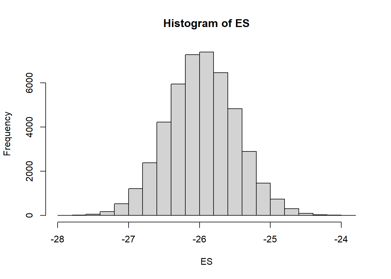

> 
> # Probability that the effect is greater than 10% (a decline of >10%)
> sum(-1 * ES > 10)/length(ES)
[1] 1
> # Probability that the effect is greater than 25% (a decline of >25%)
> sum(-1 * ES > 25)/length(ES)
[1] 0.9741304

We have defined two additional probability derivatives, both of which utilize the step function (which generates a binary vector based on whether values evaluate less than zero or not).

• P0 - the probability (mean of 1-step()) that the raw effect is greater than zero.
• P25 - the probability (mean of 1-step()) that the percent effect size is greater than \(25\)%.

> paramsv3 <- c("beta0", "beta", "sigma", "Group.means", "cohenD", "ES", "P0", "P25")
> data.r2jagsv3 <- jags(data=data.list,
+ inits=NULL, #or inits=list(inits,inits) # since there are two chains
+ parameters.to.save=paramsv3,
+ model.file="ttestModelv3.txt",
+ n.chains=nChains,
+ n.iter=nIter,
+ n.burnin=burnInSteps,
+ n.thin=thinSteps)
Compiling model graph
   Resolving undeclared variables
   Allocating nodes
Graph information:
   Observed stochastic nodes: 100
   Unobserved stochastic nodes: 3
   Total graph size: 225

Initializing model
> 
> #print results
> print(data.r2jagsv3)
Inference for Bugs model at "ttestModelv3.txt", fit using jags,
 2 chains, each with 25000 iterations (first 2000 discarded)
 n.sims = 46000 iterations saved
               mu.vect sd.vect    2.5%     25%     50%     75%   97.5%  Rhat
ES             -25.964   0.489 -26.920 -26.293 -25.965 -25.637 -24.999 1.001
Group.means[1] 105.197   0.359 104.485 104.959 105.196 105.435 105.897 1.001
Group.means[2]  77.882   0.441  77.022  77.585  77.881  78.178  78.748 1.001
P0               1.000   0.000   1.000   1.000   1.000   1.000   1.000 1.000
P25              0.975   0.156   0.000   1.000   1.000   1.000   1.000 1.001
beta[1]          0.000   0.000   0.000   0.000   0.000   0.000   0.000 1.000
beta[2]        -27.315   0.568 -28.427 -27.696 -27.314 -26.935 -26.195 1.001
beta0          105.197   0.359 104.485 104.959 105.196 105.435 105.897 1.001
cohenD          -9.912   0.740 -11.385 -10.405  -9.903  -9.412  -8.477 1.001
sigma            2.770   0.200   2.411   2.631   2.758   2.896   3.198 1.001
deviance       487.202   2.492 484.364 485.378 486.557 488.334 493.696 1.001
               n.eff
ES             46000
Group.means[1] 46000
Group.means[2] 46000
P0                 1
P25            46000
beta[1]            1
beta[2]        46000
beta0          46000
cohenD         37000
sigma          27000
deviance       46000

For each parameter, n.eff is a crude measure of effective sample size,
and Rhat is the potential scale reduction factor (at convergence, Rhat=1).

DIC info (using the rule, pD = var(deviance)/2)
pD = 3.1 and DIC = 490.3
DIC is an estimate of expected predictive error (lower deviance is better).

Finite population standard deviations

It is often useful to be able to estimate the relative amount of variability associated with each predictor (or term) in a model. This can provide a sort of relative importance measure for each predictor.

In frequentist statistics, such measures are only available for so called random factors (factors whose observational levels are randomly selected to represent all possible levels rather than to represent specific treatment levels). For such random factors, the collective variances (or standard deviation) of each factor are known as the variance components. Each component can also be expressed as a percentage of the total so as to provide a percentage breakdown of the relative contributions of each scale of sampling. Frequentist approaches model random factors according to the variance they add to the model, whereas fixed factors are modelled according to their effects (deviations from reference means). The model does not seek to generalise beyond the observed levels of a given fixed factor (such as control vs treatment) and thus it apparently does not make sense to estimate the population variability between levels (which is what variance components estimate).

The notion of “fixed” and “random” factors is somewhat arbitrary and does not really have any meaning within a Bayesian context (as all parameters and thus factors are considered random). Instead, the spirit of what many consider is that the difference between fixed and random factors can be captured by conceptualising whether the levels of a factor are drawn from a finite population (from which the observed factor levels are the only ones possible) or a superpopulation (from which the observed factor levels are just a random selection of the infinite possible levels possible). Hence, variance components could be defined in terms of either finite population or superpopulation standard deviations. Superpopulation standard deviations have traditionally been used to describe the relative scale of sampling variation (e.g. where is the greatest source of variability; plots, subplots within plots, individual quadrats within subplots, …. or years, months within years, weeks within months, days within weeks, …) and are most logically applicable to factors that have a relatively large number of levels (such as spatial or temporal sampling units). On the other hand, finite population standard deviations can be used to explore the relative impact or effect of a set of (fixed) treatments.

Calculate the amount of unexplained (residual) variance absorbed by the factor. This is generated by fitting a model with (full model) and without (reduced model) the term and subtracting the standard deviations of the residuals one another.

\[ \sigma_A = \sigma_{reduced} - \sigma_{full} \]

This approach works fine for models that only include fixed factors (indeed it is somewhat analogous to the partitioning of variance employed by an ANOVA table), but cannot be used when the model includes random factors.

> data.lmFull <- lm(y ~ x, data)
> data.lmRed <- lm(y ~ 1, data)
> sd.a <- sd(data.lmRed$resid) - sd(data.lmFull$resid)
> sd.resid <- sd(data.lmFull$resid)
> sds <- c(sd.a, sd.resid)
> 100 * sds/sum(sds)
[1] 80.05772 19.94228

However, options are somewhat limiting if we want to estimate the relative impacts of a mixture of “fixed” and “random” terms. For example, we may wish to explore the relative importance of a treatment compared to the spatial and/or temporal sampling heterogeneity. The Bayesian framework provides a relatively simple way to generate both finite population and superpopulation standard deviation estimates for all factors.

• Finite populations. The standard deviations of the MCMC samples across each of the parameters associated with a factor (eg, \(\beta_1\) and \(\beta_2\) in the effects parameterisation model) provide natural estimates of the variability between group levels (and thus the finite population standard deviation).

• Superpopulation. The mechanism of defining priors also provides a mechanism for calculating infinite population standard deviations. Recall that in the means model, the prior for \(\beta_0\) specifies that each of the \(\beta_0\) values are drawn from a normal distribution with a particular mean and a certain level of precision (reciprocal of variability). We could further parameterise this prior into an estimatable mean and precision via hyperpriors \(\beta_0 \sim \text{Normal}(\mu,\tau)\), with \(\mu \sim \text{Normal}(0,1.0\text{E}-6)\) and \(\tau \sim \text{Gamma}(0.1,0.1)\). Since the normal distribution in line one above represents the distribution from which the (infinite) population means are drawn, \(\tau\) provides a direct measure of the variability of the population from which the means are drawn.

When the number of levels of a factor are large, the finite population and superpopulation standard deviation point estimates will be very similar. However, when the number of factor levels is small (such as two levels), the finite population estimate will be very precise whereas the superpopulation standard deviation estimate will be very imprecise (highly varied). For this reason, if the purpose of estimating standard deviations is to compare relative contributions of various predictors (some of which have small numbers of levels and others large), then it is best to use finite population standard deviation estimates.

> paramsv4 <- c("beta0", "beta", "sigma", "sd.a", "sd.resid", "sigma.a")
> data.r2jagsv4 <- jags(data=data.list,
+ inits=NULL, #or inits=list(inits,inits) # since there are two chains
+ parameters.to.save=paramsv4,
+ model.file="ttestModelv4.txt",
+ n.chains=nChains,
+ n.iter=nIter,
+ n.burnin=burnInSteps,
+ n.thin=thinSteps)
Compiling model graph
   Resolving undeclared variables
   Allocating nodes
Graph information:
   Observed stochastic nodes: 100
   Unobserved stochastic nodes: 4
   Total graph size: 319

Initializing model
> 
> #print results
> print(data.r2jagsv4)
Inference for Bugs model at "ttestModelv4.txt", fit using jags,
 2 chains, each with 25000 iterations (first 2000 discarded)
 n.sims = 46000 iterations saved
               mu.vect      sd.vect    2.5%     25%     50%     75%
beta[1]   0.000000e+00 0.000000e+00   0.000   0.000   0.000   0.000
beta[2]  -2.731400e+01 5.670000e-01 -28.417 -27.694 -27.314 -26.937
beta0     1.051970e+02 3.590000e-01 104.490 104.955 105.198 105.440
sd.a      1.931400e+01 4.010000e-01  18.521  19.047  19.314  19.583
sd.resid  2.751000e+00 2.000000e-02   2.737   2.738   2.743   2.755
sigma     2.769000e+00 1.990000e-01   2.411   2.629   2.757   2.895
sigma.a   1.095446e+22 1.956638e+24   0.323   1.712  13.394 440.403
deviance  4.871890e+02 2.480000e+00 484.365 485.386 486.550 488.303
                97.5%  Rhat n.eff
beta[1]         0.000 1.000     1
beta[2]       -26.193 1.001 46000
beta0         105.899 1.001 46000
sd.a           20.094 1.001 46000
sd.resid        2.808 1.001 46000
sigma           3.187 1.001 46000
sigma.a  43469187.743 1.001 46000
deviance      493.637 1.001 46000

For each parameter, n.eff is a crude measure of effective sample size,
and Rhat is the potential scale reduction factor (at convergence, Rhat=1).

DIC info (using the rule, pD = var(deviance)/2)
pD = 3.1 and DIC = 490.3
DIC is an estimate of expected predictive error (lower deviance is better).

The between group (finite population) standard deviation is \(20.1\) whereas the within group standard deviation is \(2.81\). These equate to respectively. Compared to the finite population standard deviation, the superpopulation between group standard deviation estimate (\(\sigma_a\)) is both very large and highly variable. This is to be expected, whilst the finite population standard deviation represents the degree of variation between the observed levels, the superpopulation standard deviation seeks to estimate the variability of the population from which the group means of the observed levels AND all other possible levels are drawn. There are only two levels from which to estimate this standard deviation and therefore, its value and variability are going to be higher than those pertaining only to the scope of the current data.

Examination of the quantiles for \(\sigma_a\) suggest that its samples are not distributed normally. Consequently, the mean is not an appropriate measure of its location. We will instead characterise the superpopulation between group and within group standard deviations via their respective medians and as percent medians. The contrast between finite population and superpopulation standard deviations is also emphasised by the respective estimates for the residuals. The residuals are of course a “random” factor with a large number of observed levels. It is therefore not surprising that the point estimates for the residuals variance components are very similar. However, also notice that the precision of the finite population standard deviation estimate is substantially higher (lower standard deviation of the standard deviation estimate) than that of the superpopulation estimate.

Unequally varied populations

We can also generate data assuming two populations with different variances, e.g. between male and female subgroups.

> set.seed(123)
> n1 <- 60  #sample size from population 1
> n2 <- 40  #sample size from population 2
> mu1 <- 105  #population mean of population 1
> mu2 <- 77.5  #population mean of population 2
> sigma1 <- 3  #standard deviation of population 1
> sigma2 <- 2  #standard deviation of population 2
> n <- n1 + n2  #total sample size
> y1 <- rnorm(n1, mu1, sigma1)  #population 1 sample
> y2 <- rnorm(n2, mu2, sigma2)  #population 2 sample
> y <- c(y1, y2)
> x <- factor(rep(c("A", "B"), c(n1, n2)))  #categorical listing of the populations
> xn <- rep(c(0, 1), c(n1, n2))  #numerical version of the population category
> data2 <- data.frame(y, x, xn)  # dataset
> head(data2)  #print out the first six rows of the data set
         y x xn
1 103.3186 A  0
2 104.3095 A  0
3 109.6761 A  0
4 105.2115 A  0
5 105.3879 A  0
6 110.1452 A  0

Start by defining the model

\[ y_i = \beta_0 + \beta_1x_i + \epsilon, \]

where \(\epsilon_1 \sim \text{Normal}(0,\sigma_1)\) for \(x_1=0\) (females), and \(\epsilon_2 \sim \text{Normal}(0,\sigma_2)\) for \(x_2=1\) (males). In JAGS code, the model becomes:

> modelStringv5="
+  model {
+  #Likelihood
+  for (i in 1:n1) {
+  y1[i]~dnorm(mu1,tau1)
+  }
+  for (i in 1:n2) {
+  y2[i]~dnorm(mu2,tau2)
+  }
+  
+  #Priors
+  mu1 ~ dnorm (0,0.001)
+  mu2 ~ dnorm(0,0.001)
+  tau1 <- 1 / (sigma1 * sigma1)
+  sigma1~dunif(0,100)
+  tau2 <- 1 / (sigma2 * sigma2)
+  sigma2~dunif(0,100)
+  
+  #Other Derived parameters 
+  delta <- mu2 - mu1
+  }
+  "
> ## write the model to a text file 
> writeLines(modelStringv5,con="ttestModelv5.txt")

We specify priors directly on \(\sigma_1\) and \(\sigma_2\) using Uniform distributions between \(0\) and \(100\), and then express \(\tau\) as a deterministic function of \(\sigma\). Next, arrange the data as a list (as required by JAGS) and define the MCMC parameters. Note, all variables must be numeric, therefore we use the numeric version of \(x\). Define the initial values for two chains so that the initial values list must include two elements (if provided).

> data2.list <- with(data2,list(y1=y[xn==0], y2=y[xn==1], 
+   n1=length(y[xn==0]), n2=length(y[xn==1])))
> inits <- list(list(mu1=rnorm(1), mu2=rnorm(1), sigma1=rlnorm(1), sigma2=rlnorm(1)),
+ list(mu1=rnorm(1), mu2=rnorm(1), sigma1=rlnorm(1), sigma2=rlnorm(1)))
> paramsv5 <- c("mu1","mu2","delta","sigma1","sigma2")
> adaptSteps = 1000
> burnInSteps = 2000
> nChains = 2
> numSavedSteps = 50000
> thinSteps = 1
> nIter = ceiling((numSavedSteps * thinSteps)/nChains)

Finally, fit the model in JAGS and print the results.

> data2.r2jagsv5 <- jags(data=data2.list,
+ inits=NULL, #or inits=list(inits,inits) # since there are two chains
+ parameters.to.save=paramsv5,
+ model.file="ttestModelv5.txt",
+ n.chains=nChains,
+ n.iter=nIter,
+ n.burnin=burnInSteps,
+ n.thin=1)
Compiling model graph
   Resolving undeclared variables
   Allocating nodes
Graph information:
   Observed stochastic nodes: 100
   Unobserved stochastic nodes: 4
   Total graph size: 115

Initializing model
> 
> print(data2.r2jagsv5)
Inference for Bugs model at "ttestModelv5.txt", fit using jags,
 2 chains, each with 25000 iterations (first 2000 discarded)
 n.sims = 46000 iterations saved
         mu.vect sd.vect    2.5%     25%     50%     75%   97.5%  Rhat n.eff
delta    -27.435   0.473 -28.367 -27.755 -27.433 -27.116 -26.508 1.001 27000
mu1      105.181   0.360 104.478 104.937 105.181 105.422 105.891 1.001 44000
mu2       77.746   0.306  77.142  77.543  77.748  77.948  78.347 1.001 46000
sigma1     2.787   0.265   2.328   2.602   2.767   2.951   3.361 1.001 16000
sigma2     1.913   0.225   1.534   1.753   1.893   2.049   2.414 1.001 21000
deviance 455.879   2.945 452.217 453.714 455.215 457.354 463.257 1.001 46000

For each parameter, n.eff is a crude measure of effective sample size,
and Rhat is the potential scale reduction factor (at convergence, Rhat=1).

DIC info (using the rule, pD = var(deviance)/2)
pD = 4.3 and DIC = 460.2
DIC is an estimate of expected predictive error (lower deviance is better).