Multiple Linear Regression (Stan)
This tutorial will focus on the use of Bayesian estimation to fit simple linear regression models. BUGS (Bayesian inference Using Gibbs Sampling) is an algorithm and supporting language (resembling R) dedicated to performing the Gibbs sampling implementation of Markov Chain Monte Carlo (MCMC) method. Dialects of the BUGS language are implemented within three main projects:
OpenBUGS - written in component pascal.
JAGS - (Just Another Gibbs Sampler) - written in
C++.Stan - a dedicated Bayesian modelling framework written in
C++and implementing Hamiltonian MCMC samplers.
Whilst the above programs can be used stand-alone, they do offer the rich data pre-processing and graphical capabilities of R, and thus, they are best accessed from within R itself. As such there are multiple packages devoted to interfacing with the various software implementations:
R2OpenBUGS - interfaces with
OpenBUGSR2jags - interfaces with
JAGSrstan - interfaces with
Stan
This tutorial will demonstrate how to fit models in Stan (Gelman, Lee, and Guo (2015)) using the package rstan (Stan Development Team (2018)) as interface, which also requires to load some other packages.
Overview
Introduction
Multiple regression is an extension of simple linear regression whereby a response variable is modelled against a linear combination of two or more simultaneously measured predictor variables. There are two main purposes of multiple linear regression:
To develop a better predictive model (equation) than is possible from models based on single independent variables.
To investigate the relative individual effects of each of the multiple independent variables above and beyond (standardised across) the effects of the other variables.
Although the relationship between response variable and the additive effect of all the predictor variables is represented overall by a single multidimensional plane (surface), the individual effects of each of the predictor variables on the response variable (standardised across the other variables) can be depicted by single partial regression lines. The slope of any single partial regression line (partial regression slope) thereby represents the rate of change or effect of that specific predictor variable (holding all the other predictor variables constant to their respective mean values) on the response variable. In essence, it is the effect of one predictor variable at one specific level (the means) of all the other predictor variables (i.e. when each of the other predictors are set to their averages).
Multiple regression models can be constructed additively (containing only the predictor variables themselves) or in a multiplicative design (which incorporate interactions between predictor variables in addition to the predictor variables themselves). Multiplicative models are used primarily for testing inferences about the effects of various predictor variables and their interactions on the response variable. Additive models by contrast are used for generating predictive models and estimating the relative importance of individual predictor variables more so than hypothesis testing.
Additive Model
\[ y_i = \beta_0 + \beta_1x_{i1} + \beta_2x_{i2} + \ldots + \beta_Jx_{iJ} + \epsilon_i,\]
where \(\beta_0\) is the population \(y\)-intercept (value of \(y\) when all partial slopes equal zero), \(\beta_1,\beta_2,\ldots,\beta_{J}\) are the partial population slopes of \(Y\) on \(X_1,X_2,\ldots,X_J\) respectively holding the other \(X\) constant. \(\epsilon_i\) is the random unexplained error or residual component. The additive model assumes that the effect of one predictor variable (partial slope) is independent of the levels of the other predictor variables.
Multiplicative Model
\[ y_i = \beta_0 + \beta_1x_{i1} + \beta_2x_{i2} + \beta_3x_{i1}x_{i2} + \ldots + \beta_Jx_{iJ} + \epsilon_i,\]
where \(\beta_3x_{i1}x_{i2}\) is the interactive effect of \(X_1\) and \(X_2\) on \(Y\) and it examines the degree to which the effect of one of the predictor variables depends on the levels of the other predictor variable(s).
Data generation
Lets say we had set up a natural experiment in which we measured a response (\(y\)) from each of \(20\) sampling units (\(n=20\)) across a landscape. At the same time, we also measured two other continuous covariates (\(x_1\) and \(x_2\)) from each of the sampling units. As this section is mainly about the generation of artificial data (and not specifically about what to do with the data), understanding the actual details are optional and can be safely skipped.
> set.seed(123)
> n = 100
> intercept = 5
> temp = runif(n)
> nitro = runif(n) + 0.8 * temp
> int.eff = 2
> temp.eff <- 0.85
> nitro.eff <- 0.5
> res = rnorm(n, 0, 1)
> coef <- c(int.eff, temp.eff, nitro.eff, int.eff)
> mm <- model.matrix(~temp * nitro)
>
> y <- t(coef %*% t(mm)) + res
> data <- data.frame(y, x1 = temp, x2 = nitro, cx1 = scale(temp,
+     scale = F), cx2 = scale(nitro, scale = F))
> head(data)
         y        x1        x2         cx1         cx2
1 2.426468 0.2875775 0.8300510 -0.21098147 -0.08302110
2 4.927690 0.7883051 0.9634676  0.28974614  0.05039557
3 3.176118 0.4089769 0.8157946 -0.08958207 -0.09727750
4 6.166652 0.8830174 1.6608878  0.38445841  0.74781568
5 4.788890 0.9404673 1.2352762  0.44190829  0.32220415
6 2.541536 0.0455565 0.9267954 -0.45300249  0.01372335
With these sort of data, we are primarily interested in investigating whether there is a relationship between the continuous response variable and the components linear predictor (continuous predictors). We could model the relationship via either:
An additive model in which the effects of each predictor contribute in an additive way to the response - we do not allow for an interaction as we consider an interaction either not of great importance or likely to be absent.
A multiplicative model in which the effects of each predictor and their interaction contribute to the response - we allow for the impact of one predictor to vary across the range of the other predictor.
Centering the data
When a linear model contains a covariate (continuous predictor variable) in addition to another predictor (continuous or categorical), it is nearly always advisable that the continuous predictor variables are centered prior to the analysis. Centering is a process by which the mean of a variable is subtracted from each of the values such that the scale of the variable is shifted so as to be centered around \(0\). Hence the mean of the new centered variable will be \(0\), yet it will retain the same variance.
There are multiple reasons for this:
It provides some clinical meaning to the \(y\)-intercept. Recall that the \(y\)-intercept is the value of \(Y\) when \(X\) is equal to zero. If \(X\) is centered, then the \(y\)-intercept represents the value of \(Y\) at the mid-point of the \(X\) range. The \(y\)-intercept of an uncentered \(X\) typically represents a unreal value of \(Y\) (as an \(X\) of \(0\) is often beyond the reasonable range of values).
In multiplicative models (in which predictors and their interactions are included), main effects and interaction terms built from centered predictors will not be correlated to one another.
For more complex models, centering the covariates can increase the likelihood that the modelling engine converges (arrives at a numerically stable and reliable outcome).
Note, centering will not effect the slope estimates. In R, centering is easily achieved with the scale function, which centers and scales (divides by standard deviation) the data. We only really need to center the data, so we provide the argument scale=FALSE. Also note that the scale function attaches the pre-centered mean (and standard deviation if scaling is performed) as attributes to the scaled data in order to facilitate back-scaling to the original scale. While these attributes are often convenient, they do cause issues for some of the Bayesian routines and so we will strip these attributes using the as.numeric function. Instead, we will create separate scalar variables to store the pre-scaled means.
> data <- within(data, {
+     cx1 <- as.numeric(scale(x1, scale = FALSE))
+     cx2 <- as.numeric(scale(x2, scale = FALSE))
+ })
> head(data)
         y        x1        x2         cx1         cx2
1 2.426468 0.2875775 0.8300510 -0.21098147 -0.08302110
2 4.927690 0.7883051 0.9634676  0.28974614  0.05039557
3 3.176118 0.4089769 0.8157946 -0.08958207 -0.09727750
4 6.166652 0.8830174 1.6608878  0.38445841  0.74781568
5 4.788890 0.9404673 1.2352762  0.44190829  0.32220415
6 2.541536 0.0455565 0.9267954 -0.45300249  0.01372335
>
> mean.x1 = mean(data$x1)
> mean.x2 = mean(data$x2)
Assumptions
The assumptions of the model are:
All of the observations are independent - this must be addressed at the design and collection stages.
The response variable (and thus the residuals) should be normally distributed. A boxplot of the entire variable is usually useful for diagnosing major issues with normality.
The response variable should be equally varied (variance should not be related to mean as these are supposed to be estimated separately). Scatterplots with linear smoothers can be useful for exploring the spread of observations around the trendline. The spread of observations around the trendline should not increase (or decrease) along its length.
The predictor variables should be uniformly or normally distributed. Again, boxplots can be useful.
The relationships between the linear predictors (right hand side of the regression formula) and the response variable should be linear. Scatterplots with smoothers can be useful for identifying possible non-linearity.
(Multi)collinearity. The number of predictor variables must be less than the number of observations otherwise the linear model will be over-parameterized (more parameters to estimate than there are independent data from which estimates are calculated).
(Multi)collinearity breaks the assumption that a predictor variable must not be correlated to the combination of other predictor variables (known collectively as the linear predictor). Multicollinearity has major detrimental effects on model fitting:
Instability of the estimated partial regression slopes (small changes in the data or variable inclusion can cause dramatic changes in parameter estimates).
Inflated standard errors and confidence intervals of model parameters, thereby increasing the type II error rate (reducing power) of parameter hypothesis tests.
Multicollinearity can be diagnosed with the following situatons:
Investigate pairwise correlations between all the predictor variables either by a correlation matrix or a scatterplot matrix
Calculate the tolerance \((1−r^2)\) of the relationship between a predictor variable and all the other predictor variables for each of the predictor variables. Tolerance is a measure of the degree of collinearity and values less than \(0.2\) should be considered and values less than \(0.1\) should be given serious attention. Variance inflation factor (VIF) is the inverse of tolerance and thus values greater than \(5\), or worse, \(10\) indicate collinearity.
PCA (principle components analysis) eigenvalues (from a correlation matrix for all the predictor variables) close to zero indicate collinearity and component loadings may be useful in determining which predictor variables cause collinearity.
There are several approaches to dealing with collinearity (however the first two of these are likely to result in biased parameter estimates):
Remove the highly correlated predictor variable(s), starting with the least most clinically interesting variable(s)
PCA (principle components analysis) regression - regress the response variable against the principal components resulting from a correlation matrix for all the predictor variables. Each of these principal components by definition are completely independent, but the resulting parameter estimates must be back-calculated in order to have any clinical meaning.
Apply a regression tree - regression trees recursively partitioning (subsetting) the data in accordance to individual variables that explain the greatest remaining variance. Since at each iteration, each predictor variable is effectively evaluated in isolation, (multi)collinearity is not an issue.
Model fitting
Multiple linear regression models can include predictors (terms) that are incorporated additively (no interactions) or multiplicatively (with interactions). As such we will explore these separately for each modelling tool. The observed responses (\(y_i\)) are assumed to be drawn from a normal distribution with a given mean (\(\mu\)) and standard deviation (\(\sigma\)). The expected values are themselves determined by the linear predictor. In this case, \(\beta_0\) represents the \(y\)-intercept (value of \(y\) when all of the \(x\)’s are equal to zero) and the set of \(\beta\)’s represent the rates of change in y for every unit change in each \(x\) (the effect) holding each other \(x\) constant. Note that since we should always center all predictors (by subtracting the mean of each \(x\) from the repective values of each \(x\)), the \(y\)-intercept represents the value of \(y\) at the average value of each \(x\).
MCMC sampling requires priors on all parameters. We will employ weakly informative priors. Specifying “uninformative” priors is always a bit of a balancing act. If the priors are too vague (wide) the MCMC sampler can wander off into nonscence areas of likelihood rather than concentrate around areas of highest likelihood (desired when wanting the outcomes to be largely driven by the data). On the other hand, if the priors are too strong, they may have an influence on the parameters. In such a simple model, this balance is very forgiving - it is for more complex models that prior choice becomes more important. For this simple model, we will go with zero-centered Gaussian (normal) priors with relatively large standard deviations (\(100\)) for both the intercept and the treatment effect and a wide half-cauchy (\(\text{scale}=5\)) for the standard deviation:
\[ y_i \sim \text{Normal}(\mu_i, \sigma),\]
where \(\mu_i=\beta_0 + \boldsymbol \beta \boldsymbol X_i\). Priors are specified as: \(\boldsymbol \beta \sim \text{Normal}(0,1000)\) and \(\sigma \sim \text{Cauchy}(0,5)\). We will explore Bayesian modelling of multiple linear regression using Stan. The minimum model in Stan required to fit the above simple regression follows. Note the following modifications from the model defined in JAGS:
The normal distribution is defined by standard deviation rather than precision
Rather than using a uniform prior for \(\sigma\), I am using a half-Cauchy
Additive model
We now translate the likelihood for the additive model into Stan code.
> modelString = "
+   data {
+   int<lower=1> n;   // total number of observations
+   vector[n] Y;      // response variable
+   int<lower=1> nX;  // number of effects
+   matrix[n, nX] X;   // model matrix
+   }
+   transformed data {
+   matrix[n, nX - 1] Xc;  // centered version of X
+   vector[nX - 1] means_X;  // column means of X before centering
+
+   for (i in 2:nX) {
+   means_X[i - 1] = mean(X[, i]);
+   Xc[, i - 1] = X[, i] - means_X[i - 1];
+   }
+   }
+   parameters {
+   vector[nX-1] beta;  // population-level effects
+   real cbeta0;  // center-scale intercept
+   real<lower=0> sigma;  // residual SD
+   }
+   transformed parameters {
+   }
+   model {
+   vector[n] mu;
+   mu = Xc * beta + cbeta0;
+   // prior specifications
+   beta ~ normal(0, 100);
+   cbeta0 ~ normal(0, 100);
+   sigma ~ cauchy(0, 5);
+   // likelihood contribution
+   Y ~ normal(mu, sigma);
+   }
+   generated quantities {
+   real beta0;  // population-level intercept
+   vector[n] log_lik;
+   beta0 = cbeta0 - dot_product(means_X, beta);
+   for (i in 1:n) {
+   log_lik[i] = normal_lpdf(Y[i] | Xc[i] * beta + cbeta0, sigma);
+   }
+   }
+
+   "
> ## write the model to a stan file
> writeLines(modelString, con = "linregModeladd.stan")
> writeLines(modelString, con = "linregModelmult.stan")
Arrange the data as a list (as required by Stan). As input, Stan will need to be supplied with: the response variable, the predictor variable, the total number of observed items. This all needs to be contained within a list object. We will create two data lists, one for each of the hypotheses.
> X = model.matrix(~cx1 + cx2, data = data)
> data.list <- with(data, list(Y = y, X = X, nX = ncol(X), n = nrow(data)))
Define the nodes (parameters and derivatives) to monitor and chain parameters.
> params <- c("beta","beta0", "cbeta0", "sigma", "log_lik")
> nChains = 2
> burnInSteps = 1000
> thinSteps = 1
> numSavedSteps = 3000  #across all chains
> nIter = ceiling(burnInSteps + (numSavedSteps * thinSteps)/nChains)
> nIter
[1] 2500
Now compile and run the Stan code via the rstan interface. Note that the first time stan is run after the rstan package is loaded, it is often necessary to run any kind of randomization function just to initiate the .Random.seed variable.
> library(rstan)During the warmup stage, the No-U-Turn sampler (NUTS) attempts to determine the optimum stepsize - the stepsize that achieves the target acceptance rate (\(0.8\) or \(80\)% by default) without divergence (occurs when the stepsize is too large relative to the curvature of the log posterior and results in approximations that are likely to diverge and be biased) - and without hitting the maximum treedepth (\(10\)). At each iteration of the NUTS algorithm, the number of leapfrog steps doubles (as it increases the treedepth) and only terminates when either the NUTS criterion are satisfied or the tree depth reaches the maximum (\(10\) by default).
> data.rstan.add <- stan(data = data.list, file = "linregModeladd.stan", chains = nChains, pars = params,
+     iter = nIter, warmup = burnInSteps, thin = thinSteps, save_dso = TRUE)

SAMPLING FOR MODEL 'linregModeladd' NOW (CHAIN 1).
Chain 1:
Chain 1: Gradient evaluation took 0 seconds
Chain 1: 1000 transitions using 10 leapfrog steps per transition would take 0 seconds.
Chain 1: Adjust your expectations accordingly!
Chain 1:
Chain 1:
Chain 1: Iteration:    1 / 2500 [  0%]  (Warmup)
Chain 1: Iteration:  250 / 2500 [ 10%]  (Warmup)
Chain 1: Iteration:  500 / 2500 [ 20%]  (Warmup)
Chain 1: Iteration:  750 / 2500 [ 30%]  (Warmup)
Chain 1: Iteration: 1000 / 2500 [ 40%]  (Warmup)
Chain 1: Iteration: 1001 / 2500 [ 40%]  (Sampling)
Chain 1: Iteration: 1250 / 2500 [ 50%]  (Sampling)
Chain 1: Iteration: 1500 / 2500 [ 60%]  (Sampling)
Chain 1: Iteration: 1750 / 2500 [ 70%]  (Sampling)
Chain 1: Iteration: 2000 / 2500 [ 80%]  (Sampling)
Chain 1: Iteration: 2250 / 2500 [ 90%]  (Sampling)
Chain 1: Iteration: 2500 / 2500 [100%]  (Sampling)
Chain 1:
Chain 1:  Elapsed Time: 0.068 seconds (Warm-up)
Chain 1:                0.082 seconds (Sampling)
Chain 1:                0.15 seconds (Total)
Chain 1:

SAMPLING FOR MODEL 'linregModeladd' NOW (CHAIN 2).
Chain 2:
Chain 2: Gradient evaluation took 0 seconds
Chain 2: 1000 transitions using 10 leapfrog steps per transition would take 0 seconds.
Chain 2: Adjust your expectations accordingly!
Chain 2:
Chain 2:
Chain 2: Iteration:    1 / 2500 [  0%]  (Warmup)
Chain 2: Iteration:  250 / 2500 [ 10%]  (Warmup)
Chain 2: Iteration:  500 / 2500 [ 20%]  (Warmup)
Chain 2: Iteration:  750 / 2500 [ 30%]  (Warmup)
Chain 2: Iteration: 1000 / 2500 [ 40%]  (Warmup)
Chain 2: Iteration: 1001 / 2500 [ 40%]  (Sampling)
Chain 2: Iteration: 1250 / 2500 [ 50%]  (Sampling)
Chain 2: Iteration: 1500 / 2500 [ 60%]  (Sampling)
Chain 2: Iteration: 1750 / 2500 [ 70%]  (Sampling)
Chain 2: Iteration: 2000 / 2500 [ 80%]  (Sampling)
Chain 2: Iteration: 2250 / 2500 [ 90%]  (Sampling)
Chain 2: Iteration: 2500 / 2500 [100%]  (Sampling)
Chain 2:
Chain 2:  Elapsed Time: 0.058 seconds (Warm-up)
Chain 2:                0.085 seconds (Sampling)
Chain 2:                0.143 seconds (Total)
Chain 2:
>
> data.rstan.add
Inference for Stan model: linregModeladd.
2 chains, each with iter=2500; warmup=1000; thin=1;
post-warmup draws per chain=1500, total post-warmup draws=3000.

               mean se_mean   sd   2.5%    25%    50%    75%  97.5% n_eff Rhat
beta[1]        2.84    0.01 0.44   1.97   2.54   2.84   3.12   3.71  2285    1
beta[2]        1.59    0.01 0.38   0.84   1.34   1.59   1.85   2.34  2142    1
beta0          3.80    0.00 0.10   3.61   3.73   3.79   3.86   3.98  2801    1
cbeta0         3.80    0.00 0.10   3.61   3.73   3.79   3.86   3.98  2801    1
sigma          0.99    0.00 0.07   0.87   0.94   0.99   1.04   1.14  2556    1
log_lik[1]    -1.13    0.00 0.09  -1.31  -1.18  -1.12  -1.06  -0.96  2775    1
log_lik[2]    -0.95    0.00 0.08  -1.11  -1.00  -0.95  -0.89  -0.80  2179    1
log_lik[3]    -0.94    0.00 0.07  -1.08  -0.99  -0.94  -0.89  -0.80  2523    1
log_lik[4]    -0.95    0.00 0.09  -1.14  -1.00  -0.94  -0.88  -0.79  2242    1
log_lik[5]    -1.24    0.00 0.15  -1.58  -1.33  -1.22  -1.13  -0.98  2903    1
log_lik[6]    -0.93    0.00 0.08  -1.09  -0.99  -0.93  -0.88  -0.79  2241    1
log_lik[7]    -1.26    0.00 0.16  -1.61  -1.35  -1.25  -1.15  -1.00  2266    1
log_lik[8]    -2.01    0.01 0.28  -2.63  -2.19  -1.99  -1.81  -1.53  3096    1
log_lik[9]    -1.00    0.00 0.07  -1.14  -1.04  -0.99  -0.95  -0.86  2524    1
log_lik[10]   -1.43    0.00 0.18  -1.82  -1.54  -1.41  -1.31  -1.13  2355    1
log_lik[11]   -0.94    0.00 0.09  -1.14  -1.00  -0.94  -0.88  -0.79  2065    1
log_lik[12]   -1.14    0.00 0.10  -1.35  -1.20  -1.13  -1.07  -0.97  2388    1
log_lik[13]   -2.48    0.01 0.39  -3.30  -2.73  -2.46  -2.20  -1.77  2110    1
log_lik[14]   -0.93    0.00 0.08  -1.08  -0.98  -0.93  -0.88  -0.79  2304    1
log_lik[15]   -1.16    0.00 0.13  -1.45  -1.24  -1.15  -1.07  -0.94  2498    1
log_lik[16]   -0.95    0.00 0.09  -1.15  -1.00  -0.95  -0.89  -0.80  1914    1
log_lik[17]   -0.95    0.00 0.08  -1.10  -1.00  -0.95  -0.89  -0.80  2466    1
log_lik[18]   -1.15    0.00 0.17  -1.54  -1.25  -1.13  -1.03  -0.89  2278    1
log_lik[19]   -1.24    0.00 0.10  -1.45  -1.30  -1.24  -1.18  -1.07  2815    1
log_lik[20]   -1.34    0.00 0.18  -1.74  -1.45  -1.32  -1.21  -1.04  2830    1
log_lik[21]   -0.99    0.00 0.09  -1.21  -1.05  -0.98  -0.93  -0.83  2853    1
log_lik[22]   -1.43    0.00 0.14  -1.73  -1.52  -1.42  -1.33  -1.18  2467    1
log_lik[23]   -1.07    0.00 0.09  -1.25  -1.12  -1.06  -1.01  -0.90  2434    1
log_lik[24]   -0.97    0.00 0.09  -1.17  -1.02  -0.96  -0.90  -0.81  2261    1
log_lik[25]   -2.60    0.01 0.28  -3.21  -2.77  -2.58  -2.41  -2.11  2595    1
log_lik[26]   -1.05    0.00 0.13  -1.36  -1.13  -1.04  -0.96  -0.85  2335    1
log_lik[27]   -0.95    0.00 0.08  -1.12  -1.00  -0.94  -0.89  -0.80  2055    1
log_lik[28]   -0.93    0.00 0.08  -1.08  -0.98  -0.92  -0.87  -0.79  2120    1
log_lik[29]   -1.15    0.00 0.14  -1.45  -1.23  -1.14  -1.06  -0.93  2785    1
log_lik[30]   -0.92    0.00 0.07  -1.07  -0.97  -0.92  -0.87  -0.79  2397    1
log_lik[31]   -2.53    0.01 0.40  -3.39  -2.78  -2.50  -2.26  -1.82  3103    1
log_lik[32]   -1.34    0.00 0.22  -1.83  -1.46  -1.32  -1.18  -0.99  2880    1
log_lik[33]   -0.92    0.00 0.07  -1.07  -0.97  -0.92  -0.87  -0.79  2512    1
log_lik[34]   -0.96    0.00 0.08  -1.13  -1.01  -0.95  -0.90  -0.81  2382    1
log_lik[35]   -2.24    0.01 0.33  -2.96  -2.44  -2.21  -2.01  -1.66  3144    1
log_lik[36]   -1.55    0.00 0.13  -1.83  -1.63  -1.55  -1.46  -1.32  2554    1
log_lik[37]   -1.78    0.00 0.25  -2.33  -1.94  -1.76  -1.60  -1.35  2816    1
log_lik[38]   -1.21    0.00 0.13  -1.53  -1.29  -1.20  -1.12  -0.98  2304    1
log_lik[39]   -2.58    0.01 0.42  -3.50  -2.83  -2.55  -2.28  -1.87  2093    1
log_lik[40]   -1.69    0.00 0.18  -2.08  -1.80  -1.68  -1.57  -1.38  3172    1
log_lik[41]   -1.60    0.00 0.21  -2.07  -1.73  -1.58  -1.45  -1.24  3283    1
log_lik[42]   -0.94    0.00 0.07  -1.08  -0.99  -0.94  -0.89  -0.80  2519    1
log_lik[43]   -1.96    0.01 0.33  -2.69  -2.17  -1.94  -1.73  -1.40  2336    1
log_lik[44]   -1.86    0.00 0.24  -2.39  -2.01  -1.84  -1.69  -1.43  2578    1
log_lik[45]   -2.23    0.01 0.33  -2.95  -2.43  -2.21  -2.01  -1.64  2426    1
log_lik[46]   -0.93    0.00 0.08  -1.08  -0.98  -0.93  -0.88  -0.79  2271    1
log_lik[47]   -1.57    0.00 0.20  -2.02  -1.70  -1.56  -1.43  -1.22  2992    1
log_lik[48]   -1.23    0.00 0.16  -1.58  -1.32  -1.21  -1.11  -0.97  2201    1
log_lik[49]   -3.85    0.01 0.53  -4.99  -4.19  -3.83  -3.49  -2.91  2972    1
log_lik[50]   -1.48    0.00 0.20  -1.93  -1.60  -1.46  -1.33  -1.14  2982    1
log_lik[51]   -1.34    0.00 0.20  -1.81  -1.45  -1.31  -1.19  -1.02  2335    1
log_lik[52]   -1.23    0.00 0.08  -1.40  -1.29  -1.23  -1.17  -1.08  2737    1
log_lik[53]   -0.98    0.00 0.08  -1.15  -1.03  -0.97  -0.92  -0.83  2289    1
log_lik[54]   -1.04    0.00 0.11  -1.30  -1.11  -1.03  -0.97  -0.85  3056    1
log_lik[55]   -0.94    0.00 0.08  -1.09  -0.99  -0.94  -0.88  -0.79  2259    1
log_lik[56]   -0.92    0.00 0.07  -1.06  -0.97  -0.92  -0.87  -0.78  2382    1
log_lik[57]   -1.27    0.00 0.14  -1.56  -1.35  -1.25  -1.17  -1.03  2909    1
log_lik[58]   -1.03    0.00 0.10  -1.25  -1.09  -1.03  -0.97  -0.86  2325    1
log_lik[59]   -1.53    0.00 0.19  -1.95  -1.65  -1.51  -1.39  -1.20  2908    1
log_lik[60]   -0.95    0.00 0.08  -1.11  -1.00  -0.95  -0.90  -0.81  2495    1
log_lik[61]   -1.48    0.00 0.12  -1.74  -1.56  -1.48  -1.39  -1.26  2822    1
log_lik[62]   -1.09    0.00 0.12  -1.35  -1.16  -1.07  -1.00  -0.88  3264    1
log_lik[63]   -1.74    0.00 0.15  -2.06  -1.83  -1.73  -1.62  -1.46  2602    1
log_lik[64]   -7.03    0.02 0.92  -8.95  -7.60  -6.98  -6.37  -5.41  2823    1
log_lik[65]   -1.01    0.00 0.09  -1.20  -1.07  -1.01  -0.95  -0.85  2462    1
log_lik[66]   -0.96    0.00 0.07  -1.10  -1.01  -0.96  -0.91  -0.82  2507    1
log_lik[67]   -1.28    0.00 0.16  -1.62  -1.38  -1.27  -1.17  -1.02  3026    1
log_lik[68]   -1.09    0.00 0.11  -1.35  -1.15  -1.08  -1.01  -0.89  2351    1
log_lik[69]   -1.07    0.00 0.10  -1.27  -1.13  -1.06  -1.00  -0.89  2460    1
log_lik[70]   -1.02    0.00 0.09  -1.20  -1.07  -1.01  -0.95  -0.86  2261    1
log_lik[71]   -0.93    0.00 0.07  -1.07  -0.98  -0.93  -0.88  -0.79  2396    1
log_lik[72]   -0.92    0.00 0.07  -1.07  -0.97  -0.92  -0.87  -0.79  2216    1
log_lik[73]   -0.93    0.00 0.08  -1.09  -0.98  -0.93  -0.88  -0.79  2425    1
log_lik[74]   -3.86    0.01 0.62  -5.23  -4.26  -3.81  -3.43  -2.75  2642    1
log_lik[75]   -1.21    0.00 0.09  -1.41  -1.27  -1.21  -1.15  -1.04  2517    1
log_lik[76]   -1.41    0.00 0.14  -1.73  -1.50  -1.41  -1.31  -1.17  2875    1
log_lik[77]   -0.92    0.00 0.07  -1.07  -0.97  -0.92  -0.87  -0.79  2378    1
log_lik[78]   -0.96    0.00 0.07  -1.11  -1.01  -0.96  -0.91  -0.82  2524    1
log_lik[79]   -0.99    0.00 0.09  -1.19  -1.05  -0.99  -0.93  -0.83  2270    1
log_lik[80]   -0.94    0.00 0.08  -1.10  -0.99  -0.94  -0.89  -0.80  2576    1
log_lik[81]   -1.55    0.00 0.20  -1.97  -1.67  -1.53  -1.41  -1.19  2331    1
log_lik[82]   -1.68    0.00 0.17  -2.05  -1.78  -1.66  -1.56  -1.38  2428    1
log_lik[83]   -0.99    0.00 0.08  -1.15  -1.04  -0.99  -0.94  -0.84  2414    1
log_lik[84]   -1.37    0.00 0.16  -1.72  -1.46  -1.35  -1.26  -1.09  2425    1
log_lik[85]   -0.92    0.00 0.07  -1.07  -0.97  -0.92  -0.87  -0.79  2392    1
log_lik[86]   -0.93    0.00 0.07  -1.07  -0.98  -0.93  -0.88  -0.80  2499    1
log_lik[87]   -1.61    0.00 0.25  -2.17  -1.76  -1.59  -1.43  -1.19  2565    1
log_lik[88]   -0.96    0.00 0.09  -1.14  -1.01  -0.96  -0.90  -0.81  2598    1
log_lik[89]   -1.64    0.01 0.29  -2.29  -1.82  -1.61  -1.43  -1.17  2797    1
log_lik[90]   -1.08    0.00 0.13  -1.36  -1.16  -1.07  -0.99  -0.88  2213    1
log_lik[91]   -1.19    0.00 0.15  -1.52  -1.27  -1.17  -1.08  -0.95  2964    1
log_lik[92]   -0.99    0.00 0.08  -1.14  -1.04  -0.99  -0.93  -0.84  2422    1
log_lik[93]   -0.93    0.00 0.08  -1.09  -0.98  -0.93  -0.88  -0.79  2223    1
log_lik[94]   -1.31    0.00 0.11  -1.55  -1.38  -1.30  -1.23  -1.11  2791    1
log_lik[95]   -1.96    0.01 0.29  -2.59  -2.13  -1.93  -1.76  -1.44  2271    1
log_lik[96]   -3.54    0.01 0.45  -4.49  -3.81  -3.52  -3.21  -2.75  3044    1
log_lik[97]   -1.11    0.00 0.10  -1.33  -1.17  -1.10  -1.04  -0.93  2467    1
log_lik[98]   -1.47    0.00 0.18  -1.88  -1.59  -1.46  -1.34  -1.16  2896    1
log_lik[99]   -1.08    0.00 0.11  -1.31  -1.14  -1.07  -1.01  -0.89  2474    1
log_lik[100]  -1.65    0.00 0.13  -1.92  -1.74  -1.65  -1.56  -1.43  2754    1
lp__         -48.81    0.04 1.42 -52.32 -49.55 -48.49 -47.74 -47.03  1397    1

Samples were drawn using NUTS(diag_e) at Thu Jul 08 21:39:20 2021.
For each parameter, n_eff is a crude measure of effective sample size,
and Rhat is the potential scale reduction factor on split chains (at
convergence, Rhat=1).
Multiplicative model
We now translate the likelihood for the multiplicative model into Stan code. Arrange the data as a list (as required by Stan). As input, Stan will need to be supplied with: the response variable, the predictor variable, the total number of observed items. This all needs to be contained within a list object. We will create two data lists, one for each of the hypotheses.
> X = model.matrix(~cx1 * cx2, data = data)
> data.list <- with(data, list(Y = y, X = X, nX = ncol(X), n = nrow(data)))
Define the nodes (parameters and derivatives) to monitor and chain parameters.
> params <- c("beta","beta0", "cbeta0", "sigma", "log_lik")
> nChains = 2
> burnInSteps = 1000
> thinSteps = 1
> numSavedSteps = 3000  #across all chains
> nIter = ceiling(burnInSteps + (numSavedSteps * thinSteps)/nChains)
> nIter
[1] 2500
Now compile and run the Stan code via the rstan interface.
> data.rstan.mult <- stan(data = data.list, file = "linregModelmult.stan", chains = nChains, pars = params,
+     iter = nIter, warmup = burnInSteps, thin = thinSteps, save_dso = TRUE)

SAMPLING FOR MODEL 'linregModeladd' NOW (CHAIN 1).
Chain 1:
Chain 1: Gradient evaluation took 0 seconds
Chain 1: 1000 transitions using 10 leapfrog steps per transition would take 0 seconds.
Chain 1: Adjust your expectations accordingly!
Chain 1:
Chain 1:
Chain 1: Iteration:    1 / 2500 [  0%]  (Warmup)
Chain 1: Iteration:  250 / 2500 [ 10%]  (Warmup)
Chain 1: Iteration:  500 / 2500 [ 20%]  (Warmup)
Chain 1: Iteration:  750 / 2500 [ 30%]  (Warmup)
Chain 1: Iteration: 1000 / 2500 [ 40%]  (Warmup)
Chain 1: Iteration: 1001 / 2500 [ 40%]  (Sampling)
Chain 1: Iteration: 1250 / 2500 [ 50%]  (Sampling)
Chain 1: Iteration: 1500 / 2500 [ 60%]  (Sampling)
Chain 1: Iteration: 1750 / 2500 [ 70%]  (Sampling)
Chain 1: Iteration: 2000 / 2500 [ 80%]  (Sampling)
Chain 1: Iteration: 2250 / 2500 [ 90%]  (Sampling)
Chain 1: Iteration: 2500 / 2500 [100%]  (Sampling)
Chain 1:
Chain 1:  Elapsed Time: 0.071 seconds (Warm-up)
Chain 1:                0.089 seconds (Sampling)
Chain 1:                0.16 seconds (Total)
Chain 1:

SAMPLING FOR MODEL 'linregModeladd' NOW (CHAIN 2).
Chain 2:
Chain 2: Gradient evaluation took 0 seconds
Chain 2: 1000 transitions using 10 leapfrog steps per transition would take 0 seconds.
Chain 2: Adjust your expectations accordingly!
Chain 2:
Chain 2:
Chain 2: Iteration:    1 / 2500 [  0%]  (Warmup)
Chain 2: Iteration:  250 / 2500 [ 10%]  (Warmup)
Chain 2: Iteration:  500 / 2500 [ 20%]  (Warmup)
Chain 2: Iteration:  750 / 2500 [ 30%]  (Warmup)
Chain 2: Iteration: 1000 / 2500 [ 40%]  (Warmup)
Chain 2: Iteration: 1001 / 2500 [ 40%]  (Sampling)
Chain 2: Iteration: 1250 / 2500 [ 50%]  (Sampling)
Chain 2: Iteration: 1500 / 2500 [ 60%]  (Sampling)
Chain 2: Iteration: 1750 / 2500 [ 70%]  (Sampling)
Chain 2: Iteration: 2000 / 2500 [ 80%]  (Sampling)
Chain 2: Iteration: 2250 / 2500 [ 90%]  (Sampling)
Chain 2: Iteration: 2500 / 2500 [100%]  (Sampling)
Chain 2:
Chain 2:  Elapsed Time: 0.072 seconds (Warm-up)
Chain 2:                0.086 seconds (Sampling)
Chain 2:                0.158 seconds (Total)
Chain 2:
>
> data.rstan.mult
Inference for Stan model: linregModeladd.
2 chains, each with iter=2500; warmup=1000; thin=1;
post-warmup draws per chain=1500, total post-warmup draws=3000.

               mean se_mean   sd   2.5%    25%    50%    75%  97.5% n_eff Rhat
beta[1]        2.82    0.01 0.44   1.95   2.52   2.82   3.12   3.66  2943    1
beta[2]        1.49    0.01 0.39   0.76   1.23   1.48   1.75   2.25  2821    1
beta[3]        1.49    0.02 1.20  -0.78   0.67   1.49   2.28   3.78  3679    1
beta0          3.71    0.00 0.12   3.47   3.63   3.71   3.79   3.95  3718    1
cbeta0         3.80    0.00 0.10   3.60   3.73   3.80   3.87   3.99  3695    1
sigma          0.99    0.00 0.07   0.86   0.94   0.99   1.04   1.14  3227    1
log_lik[1]    -1.10    0.00 0.09  -1.29  -1.16  -1.10  -1.03  -0.93  3674    1
log_lik[2]    -0.97    0.00 0.09  -1.15  -1.02  -0.96  -0.91  -0.81  2804    1
log_lik[3]    -0.93    0.00 0.07  -1.07  -0.98  -0.93  -0.88  -0.79  3128    1
log_lik[4]    -0.98    0.00 0.12  -1.26  -1.03  -0.96  -0.90  -0.80  2375    1
log_lik[5]    -1.31    0.00 0.17  -1.68  -1.42  -1.30  -1.19  -1.02  3587    1
log_lik[6]    -0.94    0.00 0.08  -1.13  -0.99  -0.94  -0.89  -0.79  2326    1
log_lik[7]    -1.18    0.00 0.15  -1.53  -1.28  -1.17  -1.07  -0.93  3073    1
log_lik[8]    -2.18    0.01 0.33  -2.90  -2.39  -2.16  -1.95  -1.60  3828    1
log_lik[9]    -0.97    0.00 0.08  -1.12  -1.02  -0.97  -0.91  -0.82  3320    1
log_lik[10]   -1.45    0.00 0.18  -1.82  -1.56  -1.44  -1.32  -1.14  3178    1
log_lik[11]   -1.06    0.00 0.19  -1.56  -1.13  -1.01  -0.93  -0.82  2869    1
log_lik[12]   -1.17    0.00 0.10  -1.39  -1.23  -1.16  -1.10  -0.98  3229    1
log_lik[13]   -2.25    0.01 0.41  -3.17  -2.50  -2.21  -1.96  -1.54  3119    1
log_lik[14]   -0.93    0.00 0.08  -1.09  -0.98  -0.93  -0.88  -0.79  2507    1
log_lik[15]   -1.16    0.00 0.14  -1.45  -1.24  -1.15  -1.06  -0.93  3366    1
log_lik[16]   -0.99    0.00 0.11  -1.22  -1.05  -0.97  -0.91  -0.81  2391    1
log_lik[17]   -0.95    0.00 0.08  -1.10  -1.00  -0.95  -0.89  -0.80  2975    1
log_lik[18]   -1.08    0.00 0.16  -1.47  -1.17  -1.05  -0.97  -0.85  2736    1
log_lik[19]   -1.20    0.00 0.10  -1.42  -1.27  -1.20  -1.12  -1.01  3849    1
log_lik[20]   -1.39    0.00 0.19  -1.81  -1.51  -1.38  -1.26  -1.08  3517    1
log_lik[21]   -0.96    0.00 0.09  -1.16  -1.01  -0.95  -0.90  -0.80  2922    1
log_lik[22]   -1.34    0.00 0.15  -1.66  -1.43  -1.33  -1.23  -1.09  3406    1
log_lik[23]   -1.02    0.00 0.09  -1.21  -1.08  -1.01  -0.96  -0.85  3315    1
log_lik[24]   -0.96    0.00 0.09  -1.17  -1.01  -0.95  -0.90  -0.80  2790    1
log_lik[25]   -2.78    0.01 0.34  -3.50  -2.99  -2.76  -2.54  -2.19  3414    1
log_lik[26]   -1.08    0.00 0.14  -1.40  -1.16  -1.06  -0.98  -0.86  3266    1
log_lik[27]   -0.97    0.00 0.09  -1.17  -1.02  -0.96  -0.91  -0.81  2768    1
log_lik[28]   -0.94    0.00 0.08  -1.11  -0.99  -0.93  -0.88  -0.79  2591    1
log_lik[29]   -1.26    0.00 0.18  -1.68  -1.37  -1.24  -1.13  -0.97  3339    1
log_lik[30]   -0.93    0.00 0.08  -1.08  -0.97  -0.93  -0.88  -0.78  2722    1
log_lik[31]   -2.22    0.01 0.42  -3.16  -2.48  -2.17  -1.92  -1.52  3723    1
log_lik[32]   -1.16    0.00 0.22  -1.71  -1.27  -1.12  -1.00  -0.86  3550    1
log_lik[33]   -0.93    0.00 0.07  -1.08  -0.97  -0.93  -0.87  -0.79  2898    1
log_lik[34]   -0.98    0.00 0.09  -1.17  -1.03  -0.97  -0.91  -0.81  3177    1
log_lik[35]   -2.65    0.01 0.52  -3.76  -2.99  -2.60  -2.27  -1.80  3714    1
log_lik[36]   -1.68    0.00 0.18  -2.06  -1.80  -1.66  -1.55  -1.36  3406    1
log_lik[37]   -1.86    0.00 0.27  -2.44  -2.03  -1.84  -1.67  -1.41  3866    1
log_lik[38]   -1.30    0.00 0.17  -1.67  -1.41  -1.29  -1.18  -1.02  3197    1
log_lik[39]   -2.98    0.01 0.59  -4.27  -3.36  -2.93  -2.56  -1.96  3093    1
log_lik[40]   -1.78    0.00 0.20  -2.20  -1.91  -1.76  -1.63  -1.43  3908    1
log_lik[41]   -1.37    0.00 0.24  -1.92  -1.52  -1.35  -1.20  -1.00  3676    1
log_lik[42]   -0.93    0.00 0.07  -1.07  -0.98  -0.93  -0.88  -0.79  3178    1
log_lik[43]   -2.04    0.01 0.34  -2.79  -2.25  -2.00  -1.79  -1.46  3044    1
log_lik[44]   -1.92    0.00 0.26  -2.48  -2.08  -1.90  -1.74  -1.49  3275    1
log_lik[45]   -2.06    0.01 0.34  -2.81  -2.29  -2.03  -1.81  -1.50  3201    1
log_lik[46]   -1.00    0.00 0.13  -1.32  -1.06  -0.98  -0.91  -0.81  2511    1
log_lik[47]   -1.78    0.00 0.29  -2.40  -1.96  -1.75  -1.57  -1.31  3498    1
log_lik[48]   -1.24    0.00 0.16  -1.59  -1.33  -1.22  -1.12  -0.97  3035    1
log_lik[49]   -3.57    0.01 0.53  -4.69  -3.91  -3.55  -3.21  -2.58  3363    1
log_lik[50]   -1.63    0.00 0.25  -2.19  -1.79  -1.60  -1.45  -1.20  4046    1
log_lik[51]   -1.39    0.00 0.22  -1.87  -1.53  -1.36  -1.23  -1.03  3192    1
log_lik[52]   -1.29    0.00 0.11  -1.52  -1.37  -1.29  -1.22  -1.10  3649    1
log_lik[53]   -1.00    0.00 0.09  -1.19  -1.05  -0.99  -0.94  -0.84  2942    1
log_lik[54]   -1.26    0.00 0.25  -1.89  -1.40  -1.21  -1.08  -0.91  3271    1
log_lik[55]   -0.93    0.00 0.08  -1.09  -0.98  -0.93  -0.88  -0.79  2780    1
log_lik[56]   -0.93    0.00 0.08  -1.09  -0.98  -0.93  -0.88  -0.79  2803    1
log_lik[57]   -1.21    0.00 0.14  -1.50  -1.29  -1.19  -1.11  -0.98  3788    1
log_lik[58]   -0.99    0.00 0.10  -1.20  -1.05  -0.98  -0.92  -0.82  3036    1
log_lik[59]   -1.49    0.00 0.18  -1.91  -1.60  -1.48  -1.36  -1.17  3458    1
log_lik[60]   -0.95    0.00 0.08  -1.13  -1.00  -0.95  -0.90  -0.81  3118    1
log_lik[61]   -1.56    0.00 0.15  -1.87  -1.65  -1.56  -1.46  -1.30  3563    1
log_lik[62]   -1.29    0.00 0.24  -1.86  -1.43  -1.25  -1.12  -0.94  3390    1
log_lik[63]   -1.62    0.00 0.17  -1.98  -1.73  -1.61  -1.50  -1.33  3569    1
log_lik[64]   -6.83    0.02 0.92  -8.77  -7.42  -6.79  -6.20  -5.14  3238    1
log_lik[65]   -0.99    0.00 0.09  -1.19  -1.05  -0.99  -0.93  -0.83  3241    1
log_lik[66]   -0.99    0.00 0.08  -1.15  -1.04  -0.99  -0.94  -0.84  2924    1
log_lik[67]   -1.22    0.00 0.15  -1.54  -1.31  -1.20  -1.11  -0.97  3854    1
log_lik[68]   -1.04    0.00 0.11  -1.29  -1.10  -1.02  -0.96  -0.85  3124    1
log_lik[69]   -1.09    0.00 0.10  -1.31  -1.15  -1.08  -1.02  -0.91  3095    1
log_lik[70]   -1.03    0.00 0.09  -1.22  -1.09  -1.02  -0.97  -0.86  3101    1
log_lik[71]   -0.93    0.00 0.08  -1.08  -0.98  -0.93  -0.88  -0.78  3045    1
log_lik[72]   -0.93    0.00 0.08  -1.09  -0.98  -0.93  -0.88  -0.79  2660    1
log_lik[73]   -0.93    0.00 0.08  -1.08  -0.98  -0.93  -0.88  -0.78  2728    1
log_lik[74]   -3.71    0.01 0.62  -5.05  -4.11  -3.67  -3.28  -2.60  3558    1
log_lik[75]   -1.14    0.00 0.11  -1.37  -1.21  -1.14  -1.07  -0.96  3464    1
log_lik[76]   -1.40    0.00 0.14  -1.71  -1.49  -1.39  -1.29  -1.15  3811    1
log_lik[77]   -0.93    0.00 0.07  -1.07  -0.98  -0.93  -0.88  -0.79  2990    1
log_lik[78]   -0.99    0.00 0.08  -1.15  -1.04  -0.99  -0.94  -0.84  2929    1
log_lik[79]   -1.07    0.00 0.13  -1.36  -1.15  -1.06  -0.98  -0.86  2678    1
log_lik[80]   -0.96    0.00 0.09  -1.16  -1.02  -0.96  -0.90  -0.81  2824    1
log_lik[81]   -1.41    0.00 0.21  -1.87  -1.54  -1.39  -1.25  -1.06  3110    1
log_lik[82]   -1.81    0.00 0.22  -2.27  -1.94  -1.79  -1.66  -1.42  3361    1
log_lik[83]   -0.96    0.00 0.08  -1.12  -1.01  -0.95  -0.90  -0.81  3006    1
log_lik[84]   -1.28    0.00 0.16  -1.64  -1.37  -1.26  -1.17  -1.02  3328    1
log_lik[85]   -0.93    0.00 0.08  -1.08  -0.98  -0.93  -0.88  -0.78  2628    1
log_lik[86]   -0.92    0.00 0.07  -1.06  -0.97  -0.92  -0.87  -0.78  3077    1
log_lik[87]   -1.62    0.00 0.25  -2.18  -1.77  -1.59  -1.44  -1.20  3178    1
log_lik[88]   -0.94    0.00 0.08  -1.12  -0.99  -0.94  -0.89  -0.79  2876    1
log_lik[89]   -1.40    0.00 0.30  -2.13  -1.56  -1.35  -1.18  -0.96  3816    1
log_lik[90]   -1.02    0.00 0.12  -1.30  -1.09  -1.00  -0.93  -0.83  2616    1
log_lik[91]   -1.05    0.00 0.15  -1.40  -1.13  -1.02  -0.94  -0.83  2983    1
log_lik[92]   -0.96    0.00 0.08  -1.13  -1.01  -0.96  -0.90  -0.81  3169    1
log_lik[93]   -0.96    0.00 0.10  -1.17  -1.01  -0.95  -0.89  -0.79  2027    1
log_lik[94]   -1.26    0.00 0.11  -1.49  -1.34  -1.26  -1.19  -1.07  3811    1
log_lik[95]   -1.72    0.01 0.31  -2.41  -1.92  -1.69  -1.49  -1.21  2817    1
log_lik[96]   -3.34    0.01 0.45  -4.31  -3.63  -3.33  -3.03  -2.51  3729    1
log_lik[97]   -1.14    0.00 0.11  -1.38  -1.21  -1.13  -1.07  -0.95  3119    1
log_lik[98]   -1.53    0.00 0.20  -1.97  -1.66  -1.50  -1.38  -1.18  3713    1
log_lik[99]   -1.07    0.00 0.11  -1.30  -1.13  -1.06  -0.99  -0.89  3149    1
log_lik[100]  -1.55    0.00 0.15  -1.86  -1.65  -1.54  -1.44  -1.30  3735    1
lp__         -48.59    0.04 1.58 -52.59 -49.37 -48.26 -47.45 -46.52  1518    1

Samples were drawn using NUTS(diag_e) at Thu Jul 08 21:39:22 2021.
For each parameter, n_eff is a crude measure of effective sample size,
and Rhat is the potential scale reduction factor on split chains (at
convergence, Rhat=1).
MCMC diagnostics
In addition to the regular model diagnostic checks (such as residual plots), for Bayesian analyses, it is necessary to explore the characteristics of the MCMC chains and the sampler in general. Recall that the purpose of MCMC sampling is to replicate the posterior distribution of the model likelihood and priors by drawing a known number of samples from this posterior (thereby formulating a probability distribution). This is only reliable if the MCMC samples accurately reflect the posterior. Unfortunately, since we only know the posterior in the most trivial of circumstances, it is necessary to rely on indirect measures of how accurately the MCMC samples are likely to reflect the likelihood. I will briefly outline the most important diagnostics.
Traceplots for each parameter illustrate the MCMC sample values after each successive iteration along the chain. Bad chain mixing (characterised by any sort of pattern) suggests that the MCMC sampling chains may not have completely traversed all features of the posterior distribution and that more iterations are required to ensure the distribution has been accurately represented.
Autocorrelation plot for each parameter illustrate the degree of correlation between MCMC samples separated by different lags. For example, a lag of \(0\) represents the degree of correlation between each MCMC sample and itself (obviously this will be a correlation of \(1\)). A lag of \(1\) represents the degree of correlation between each MCMC sample and the next sample along the chain and so on. In order to be able to generate unbiased estimates of parameters, the MCMC samples should be independent (uncorrelated).
Potential scale reduction factor (Rhat) statistic for each parameter provides a measure of sampling efficiency/effectiveness. Ideally, all values should be less than \(1.05\). If there are values of \(1.05\) or greater it suggests that the sampler was not very efficient or effective. Not only does this mean that the sampler was potentially slower than it could have been but, more importantly, it could indicate that the sampler spent time sampling in a region of the likelihood that is less informative. Such a situation can arise from either a misspecified model or overly vague priors that permit sampling in otherwise nonscence parameter space.
Prior to examining the summaries, we should have explored the convergence diagnostics. We use the package mcmcplots to obtain density and trace plots for the effects model as an example.
> library(mcmcplots)
> s = as.array(data.rstan.mult)
> mcmc <- do.call(mcmc.list, plyr:::alply(s[, , -(length(s[1, 1, ]))], 2, as.mcmc))
> denplot(mcmc, parms = c("beta0","beta","cbeta0","sigma"))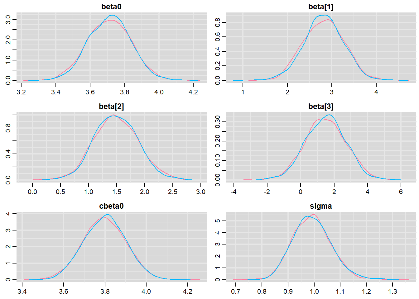
> traplot(mcmc, parms = c("beta0","beta","cbeta0","sigma"))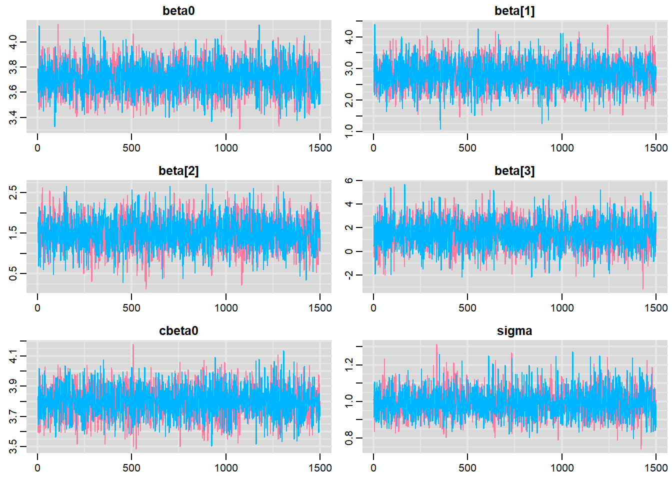
These plots show no evidence that the chains have not reasonably traversed the entire multidimensional parameter space.
> #Raftery diagnostic
> raftery.diag(mcmc)
$`1`

Quantile (q) = 0.025
Accuracy (r) = +/- 0.005
Probability (s) = 0.95

You need a sample size of at least 3746 with these values of q, r and s

$`2`

Quantile (q) = 0.025
Accuracy (r) = +/- 0.005
Probability (s) = 0.95

You need a sample size of at least 3746 with these values of q, r and s
The Raftery diagnostics for each chain estimate that we would require no more than \(5000\) samples to reach the specified level of confidence in convergence. As we have \(10500\) samples, we can be confidence that convergence has occurred.
> #Autocorrelation diagnostic
> stan_ac(data.rstan.mult, pars = c("beta","beta0"))
A lag of 10 appears to be sufficient to avoid autocorrelation (poor mixing).
> stan_ac(data.rstan.mult, pars = c("beta","beta0"))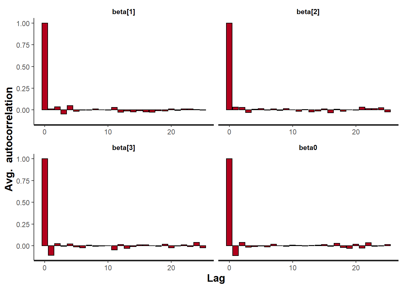
> stan_ess(data.rstan.mult, pars = c("beta","beta0"))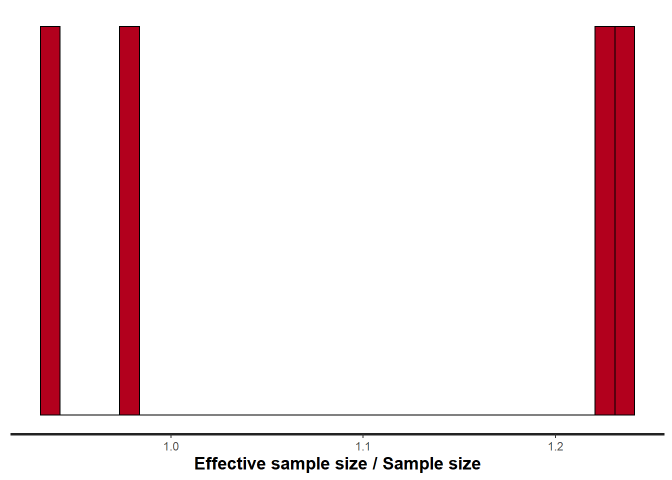
Rhat and effective sample size. In this instance, most of the parameters have reasonably high effective samples and thus there is likely to be a good range of values from which to estimate paramter properties.
Model validation
Model validation involves exploring the model diagnostics and fit to ensure that the model is broadly appropriate for the data. As such, exploration of the residuals should be routine. Ideally, a good model should also be able to predict the data used to fit the model. Residuals are not computed directly within rstan However, we can calculate them manually form the posteriors.
> library(ggplot2)
> library(dplyr)
> mcmc = as.data.frame(data.rstan.mult) %>% dplyr:::select(beta0, starts_with("beta"),
+     sigma) %>% as.matrix
> # generate a model matrix
> newdata = data
> Xmat = model.matrix(~cx1 * cx2, newdata)
> ## get median parameter estimates
> coefs = apply(mcmc[, 1:4], 2, median)
> fit = as.vector(coefs %*% t(Xmat))
> resid = data$y - fit
> ggplot() + geom_point(data = NULL, aes(y = resid, x = fit))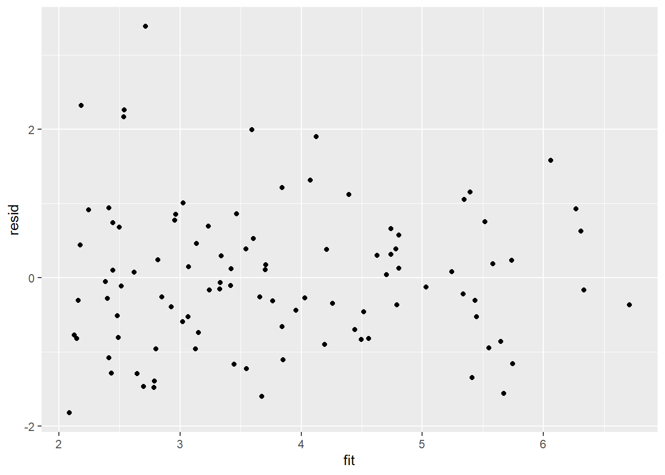
Residuals against predictors
> library(tidyr)
> mcmc = as.data.frame(data.rstan.mult) %>% dplyr:::select(beta0, starts_with("beta"),
+     sigma) %>% as.matrix
> # generate a model matrix
> newdata = newdata
> Xmat = model.matrix(~cx1 * cx2, newdata)
> ## get median parameter estimates
> coefs = apply(mcmc[, 1:4], 2, median)
> fit = as.vector(coefs %*% t(Xmat))
> resid = data$y - fit
> newdata = data %>% cbind(fit, resid)
> newdata.melt = newdata %>% gather(key = Pred, value = Value, cx1:cx2)
> ggplot(newdata.melt) + geom_point(aes(y = resid, x = Value)) + facet_wrap(~Pred)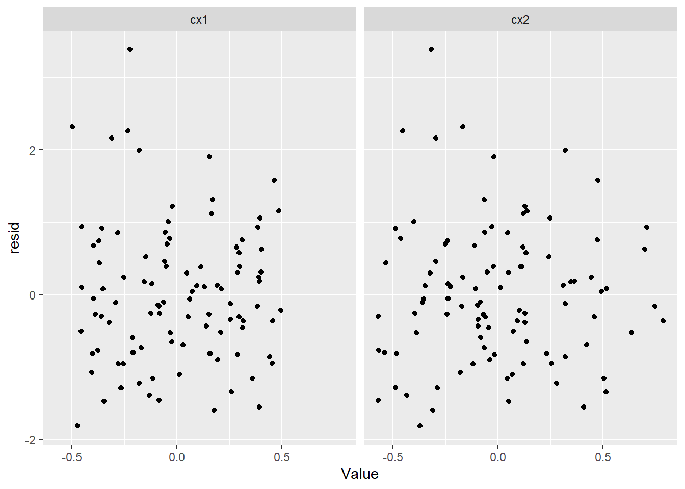
And now for studentised residuals
> mcmc = as.data.frame(data.rstan.mult) %>% dplyr:::select(beta0, starts_with("beta"),
+     sigma) %>% as.matrix
> # generate a model matrix
> newdata = data
> Xmat = model.matrix(~cx1 * cx2, newdata)
> ## get median parameter estimates
> coefs = apply(mcmc[, 1:4], 2, median)
> fit = as.vector(coefs %*% t(Xmat))
> resid = data$y - fit
> sresid = resid/sd(resid)
> ggplot() + geom_point(data = NULL, aes(y = sresid, x = fit))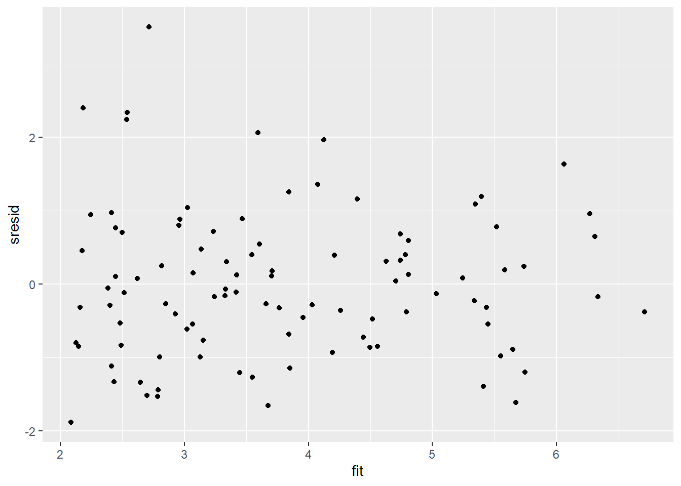
For this simple model, the studentized residuals yield the same pattern as the raw residuals (or the Pearson residuals for that matter). Lets see how well data simulated from the model reflects the raw data.
> mcmc = as.data.frame(data.rstan.mult) %>% dplyr:::select(beta0,
+     starts_with("beta"), sigma) %>% as.matrix
> # generate a model matrix
> Xmat = model.matrix(~cx1 * cx2, data)
> ## get median parameter estimates
> coefs = mcmc[, 1:4]
> fit = coefs %*% t(Xmat)
> ## draw samples from this model
> yRep = sapply(1:nrow(mcmc), function(i) rnorm(nrow(data), fit[i,
+     ], mcmc[i, "sigma"]))
> ggplot() + geom_density(data = NULL, aes(x = as.vector(yRep),
+     fill = "Model"), alpha = 0.5) + geom_density(data = data,
+     aes(x = y, fill = "Obs"), alpha = 0.5)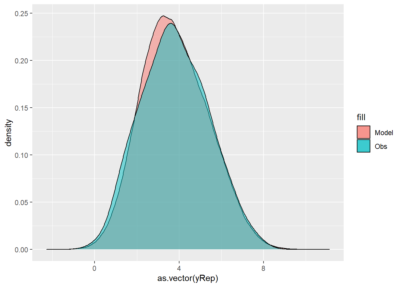
We can also explore the posteriors of each parameter.
> library(bayesplot)
> mcmc_intervals(as.matrix(data.rstan.mult), regex_pars = "beta|sigma")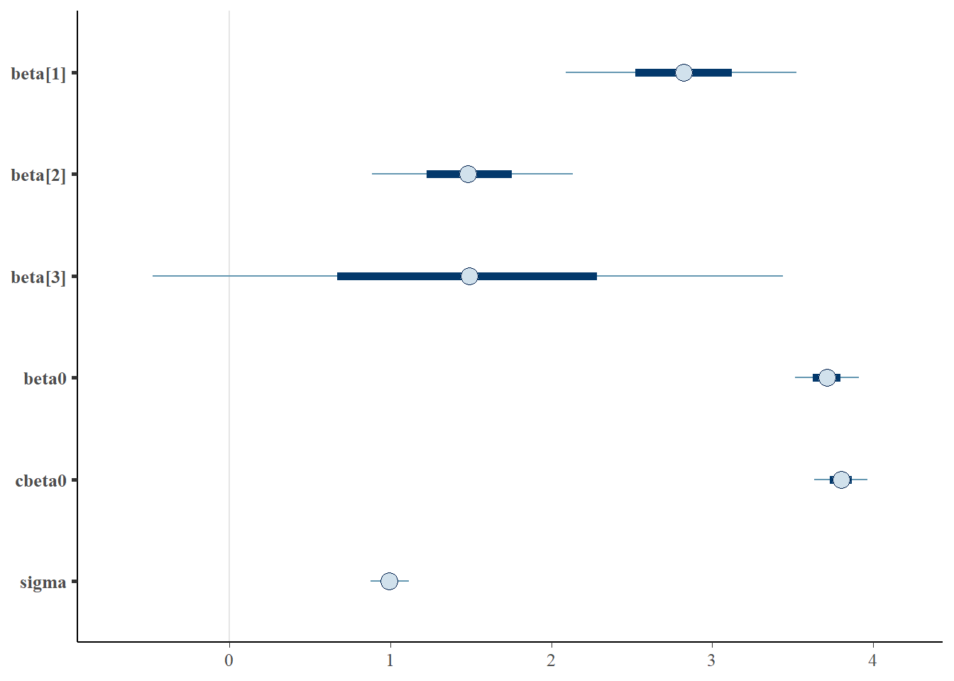
> mcmc_areas(as.matrix(data.rstan.mult), regex_pars = "beta|sigma")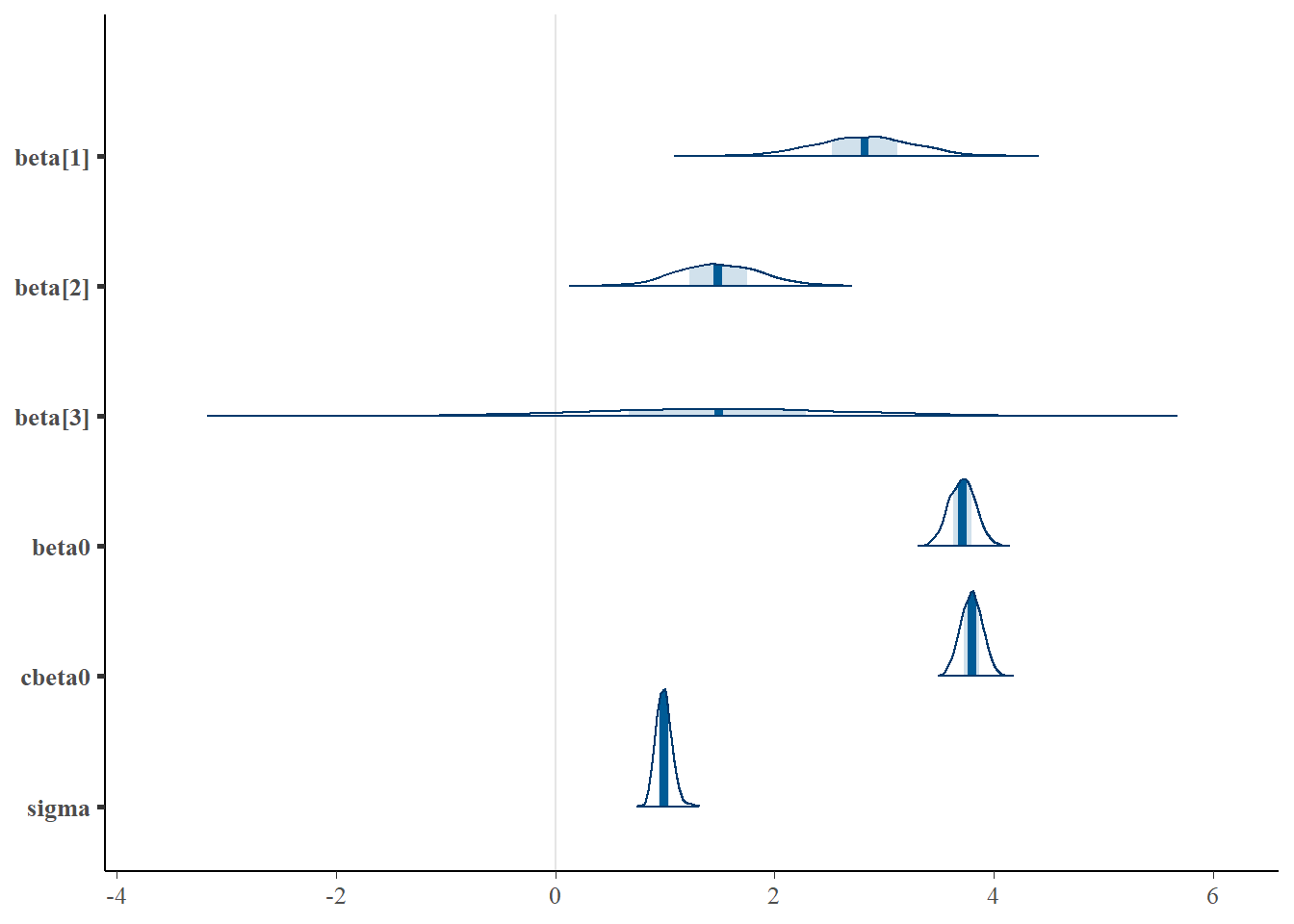
Parameter estimates
Although all parameters in a Bayesian analysis are considered random and are considered a distribution, rarely would it be useful to present tables of all the samples from each distribution. On the other hand, plots of the posterior distributions have some use. Nevertheless, most workers prefer to present simple statistical summaries of the posteriors. Popular choices include the median (or mean) and \(95\)% credibility intervals.
> mcmcpvalue <- function(samp) {
+     ## elementary version that creates an empirical p-value for the
+     ## hypothesis that the columns of samp have mean zero versus a general
+     ## multivariate distribution with elliptical contours.
+
+     ## differences from the mean standardized by the observed
+     ## variance-covariance factor
+
+     ## Note, I put in the bit for single terms
+     if (length(dim(samp)) == 0) {
+         std <- backsolve(chol(var(samp)), cbind(0, t(samp)) - mean(samp),
+             transpose = TRUE)
+         sqdist <- colSums(std * std)
+         sum(sqdist[-1] > sqdist[1])/length(samp)
+     } else {
+         std <- backsolve(chol(var(samp)), cbind(0, t(samp)) - colMeans(samp),
+             transpose = TRUE)
+         sqdist <- colSums(std * std)
+         sum(sqdist[-1] > sqdist[1])/nrow(samp)
+     }
+
+ }
First, we look at the results from the additive model.
> print(data.rstan.add, pars = c("beta0", "beta", "sigma"))
Inference for Stan model: linregModeladd.
2 chains, each with iter=2500; warmup=1000; thin=1;
post-warmup draws per chain=1500, total post-warmup draws=3000.

        mean se_mean   sd 2.5%  25%  50%  75% 97.5% n_eff Rhat
beta0   3.80    0.00 0.10 3.61 3.73 3.79 3.86  3.98  2801    1
beta[1] 2.84    0.01 0.44 1.97 2.54 2.84 3.12  3.71  2285    1
beta[2] 1.59    0.01 0.38 0.84 1.34 1.59 1.85  2.34  2142    1
sigma   0.99    0.00 0.07 0.87 0.94 0.99 1.04  1.14  2556    1

Samples were drawn using NUTS(diag_e) at Thu Jul 08 21:39:20 2021.
For each parameter, n_eff is a crude measure of effective sample size,
and Rhat is the potential scale reduction factor on split chains (at
convergence, Rhat=1).
>
> # OR
> library(broom)
> library(broom.mixed)
> tidyMCMC(data.rstan.add, conf.int = TRUE, conf.method = "HPDinterval",
+     pars = c("beta0", "beta", "sigma"))
# A tibble: 4 x 5
  term    estimate std.error conf.low conf.high
  <chr>      <dbl>     <dbl>    <dbl>     <dbl>
1 beta0      3.79     0.0970    3.61       3.98
2 beta[1]    2.84     0.441     1.97       3.70
3 beta[2]    1.59     0.382     0.845      2.34
4 sigma      0.989    0.0706    0.861      1.13
Conclusions
When
cx2is held constant, a one unit increase incx1is associated with a \(2.83\) change in \(y\). That is, \(y\) increases at a rate of \(2.83\) per unit increase incx1when standardised forcx2.When
cx1is held constant, a one unit increase incx2is associated with a \(1.58\) change in \(y\). That is, \(y\) increases at a rate of \(1.58\) per unit increase incx2when standardised forcx1.
Note, as this is an additive model, the rates associated with cx1 are assumed to be constant throughtout the range of cx2 and vice versa. The \(95\)% confidence interval for each partial slope does not overlap with \(0\) implying a significant effects of cx1 and cx2 on \(y\). While workers attempt to become comfortable with a new statistical framework, it is only natural that they like to evaluate and comprehend new structures and output alongside more familiar concepts. One way to facilitate this is via Bayesian p-values that are somewhat analogous to the frequentist p-values for investigating the hypothesis that a parameter is equal to zero.
> mcmcpvalue(as.matrix(data.rstan.add)[, "beta[1]"])
[1] 0
> mcmcpvalue(as.matrix(data.rstan.add)[, "beta[2]"])
[1] 0
With a p-value of essentially \(0\), we would conclude that there is almost no evidence that the slope was likely to be equal to zero, suggesting there is a relationship. Next, we look at the results from the multiplicative model.
> print(data.rstan.mult, pars = c("beta0", "beta", "sigma"))
Inference for Stan model: linregModeladd.
2 chains, each with iter=2500; warmup=1000; thin=1;
post-warmup draws per chain=1500, total post-warmup draws=3000.

        mean se_mean   sd  2.5%  25%  50%  75% 97.5% n_eff Rhat
beta0   3.71    0.00 0.12  3.47 3.63 3.71 3.79  3.95  3718    1
beta[1] 2.82    0.01 0.44  1.95 2.52 2.82 3.12  3.66  2943    1
beta[2] 1.49    0.01 0.39  0.76 1.23 1.48 1.75  2.25  2821    1
beta[3] 1.49    0.02 1.20 -0.78 0.67 1.49 2.28  3.78  3679    1
sigma   0.99    0.00 0.07  0.86 0.94 0.99 1.04  1.14  3227    1

Samples were drawn using NUTS(diag_e) at Thu Jul 08 21:39:22 2021.
For each parameter, n_eff is a crude measure of effective sample size,
and Rhat is the potential scale reduction factor on split chains (at
convergence, Rhat=1).
>
> # OR
> library(broom)
> tidyMCMC(data.rstan.mult, conf.int = TRUE, conf.method = "HPDinterval",
+     pars = c("beta0", "beta", "sigma"))
# A tibble: 5 x 5
  term    estimate std.error conf.low conf.high
  <chr>      <dbl>     <dbl>    <dbl>     <dbl>
1 beta0      3.71     0.122     3.48       3.96
2 beta[1]    2.82     0.444     1.93       3.61
3 beta[2]    1.48     0.385     0.765      2.26
4 beta[3]    1.49     1.20     -0.782      3.78
5 sigma      0.990    0.0726    0.854      1.13
Conclusions
At the average level of
cx2 (=0), a one unit increase incx1is associated with a \(2.80\) change in y. That is, y increases at a rate of \(2.80\) per unit increase incx1when standardised forcx2.At the average level of
cx1 (=0), a one unit increase incx2is associated with a \(1.50\) change in \(y\). That is, \(y\) increases at a rate of \(1.50\) per unit increase incx2when standardised forcx1.The degree to which the rate of change in response associated with a one unit change in
cx1changes over the range ofcx2(and vice versa) is \(1.45\).
The \(95\)% confidence intervals for the interaction partial slope does not overlap with \(0\) implying a significant interaction between cx1 and cx2. This suggests that the nature of the relationship between \(y\) and cx1 depends on the level of cx2 (and vice versa). The estimates of the effect of cx1 are only appropriate when cx2 = 0 etc. While workers attempt to become comfortable with a new statistical framework, it is only natural that they like to evaluate and comprehend new structures and output alongside more familiar concepts. One way to facilitate this is via Bayesian p-values that are somewhat analogous to the frequentist p-values for investigating the hypothesis that a parameter is equal to zero.
> ## since values are less than zero
> mcmcpvalue(as.matrix(data.rstan.mult)[, "beta[1]"])
[1] 0
> mcmcpvalue(as.matrix(data.rstan.mult)[, "beta[2]"])
[1] 0
> mcmcpvalue(as.matrix(data.rstan.mult)[, "beta[3]"])
[1] 0.215
With a p-value of essentially \(0\), we would conclude that there is almost no evidence that the slope was likely to be equal to zero, suggesting there is a relationship. An alternative way of quantifying the impact of an interaction is to compare models with and without the interactions. In a Bayesian context, this can be achieved by comparing the leave-one-out cross-validation statistics. Leave-one-out (LOO) cross-validation explores how well a series of models can predict withheld values Vehtari, Gelman, and Gabry (2017). The LOO Information Criterion (LOOIC) is analogous to the AIC except that the LOOIC takes priors into consideration, does not assume that the posterior distribution is drawn from a multivariate normal and integrates over parameter uncertainty so as to yield a distribution of looic rather than just a point estimate. The LOOIC does however assume that all observations are equally influential (it does not matter which observations are left out). This assumption can be examined via the Pareto \(k\) estimate (values greater than \(0.5\) or more conservatively \(0.75\) are considered overly influential). We can compute LOOIC if we store the loglikelihood from our Stan model, which can then be extracted to compute the information criterion using the package loo.
> ## since values are less than zero
> library(loo)
> (full = loo(extract_log_lik(data.rstan.mult)))

Computed from 3000 by 100 log-likelihood matrix

         Estimate   SE
elpd_loo   -143.2  8.5
p_loo         5.1  1.1
looic       286.3 17.0
------
Monte Carlo SE of elpd_loo is 0.1.

All Pareto k estimates are good (k < 0.5).
See help('pareto-k-diagnostic') for details.
>
> (reduced = loo(extract_log_lik(data.rstan.add)))

Computed from 3000 by 100 log-likelihood matrix

         Estimate   SE
elpd_loo   -142.9  8.7
p_loo         4.3  1.0
looic       285.8 17.4
------
Monte Carlo SE of elpd_loo is 0.0.

All Pareto k estimates are good (k < 0.5).
See help('pareto-k-diagnostic') for details.
>
> par(mfrow = 1:2, mar = c(5, 3.8, 1, 0) + 0.1, las = 3)
> plot(full, label_points = TRUE)
> plot(reduced, label_points = TRUE)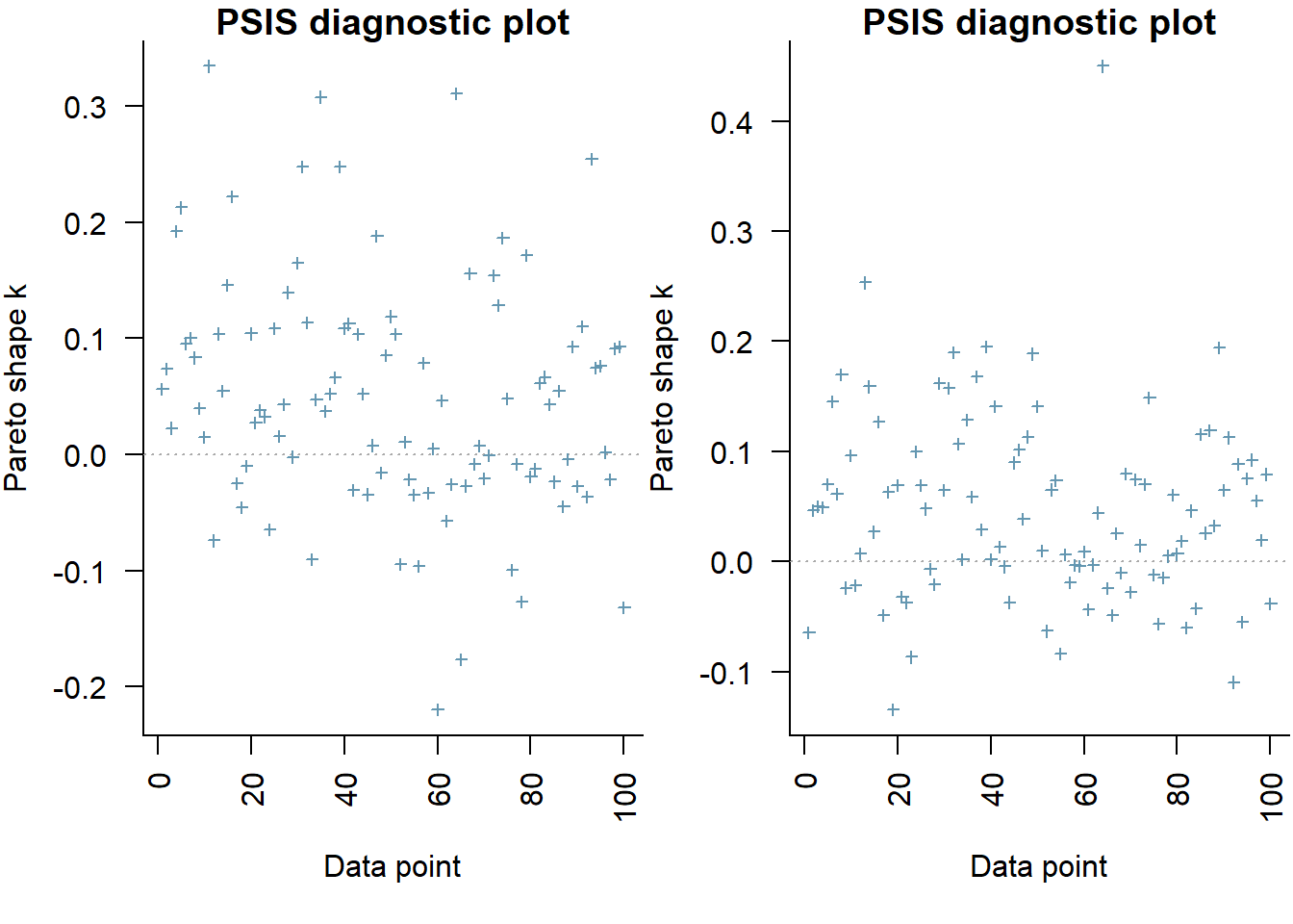
The expected out-of-sample predictive accuracy is very similar (slightly lower) for the additive model compared to the multiplicative model (model containing the interaction). This might be used to suggest that the inferential evidence for an interaction is low.
Graphical summaries
With appropriate use of model matrices and data wrangling, it is possible to produce a single prediction data set along with ggplot syntax to produce a multi-panel figure. First we look at the additive model.
> mcmc = as.matrix(data.rstan.add)
> ## Calculate the fitted values
> newdata = rbind(data.frame(cx1 = seq(min(data$cx1, na.rm = TRUE), max(data$cx1,
+     na.rm = TRUE), len = 100), cx2 = 0, Pred = 1), data.frame(cx1 = 0,
+     cx2 = seq(min(data$cx2, na.rm = TRUE), max(data$cx2, na.rm = TRUE),
+         len = 100), Pred = 2))
> Xmat = model.matrix(~cx1 + cx2, newdata)
> coefs = mcmc[, c("beta0", "beta[1]", "beta[2]")]
> fit = coefs %*% t(Xmat)
> newdata = newdata %>% mutate(x1 = cx1 + mean.x1, x2 = cx2 + mean.x2) %>%
+     cbind(tidyMCMC(fit, conf.int = TRUE, conf.method = "HPDinterval")) %>%
+     mutate(x = dplyr:::recode(Pred, x1, x2))
>
> ggplot(newdata, aes(y = estimate, x = x)) + geom_line() + geom_ribbon(aes(ymin = conf.low,
+     ymax = conf.high), fill = "blue", alpha = 0.3) + scale_y_continuous("Y") +
+     scale_x_continuous("X") + theme_classic() + facet_wrap(~Pred)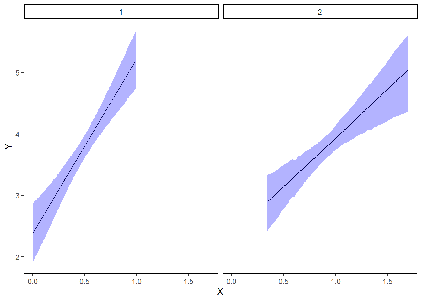
We cannot simply add the raw data to this figure. The reason for this is that the trends represent the effect of one predictor holding the other variable constant. Therefore, the observations we represent on the figure must likewise be standardised. We can achieve this by adding the partial residuals to the figure. Partial residuals are the fitted values plus the residuals.
> ## Calculate partial residuals fitted values
> fdata = rdata = rbind(data.frame(cx1 = data$cx1, cx2 = 0, Pred = 1), data.frame(cx1 = 0,
+     cx2 = data$cx2, Pred = 2))
> fMat = rMat = model.matrix(~cx1 + cx2, fdata)
> fit = as.vector(apply(coefs, 2, median) %*% t(fMat))
> resid = as.vector(data$y - apply(coefs, 2, median) %*% t(rMat))
> rdata = rdata %>% mutate(partial.resid = resid + fit) %>% mutate(x1 = cx1 +
+     mean.x1, x2 = cx2 + mean.x2) %>% mutate(x = dplyr:::recode(Pred, x1,
+     x2))
>
> ggplot(newdata, aes(y = estimate, x = x)) + geom_point(data = rdata, aes(y = partial.resid),
+     color = "gray") + geom_line() + geom_ribbon(aes(ymin = conf.low, ymax = conf.high),
+     fill = "blue", alpha = 0.3) + scale_y_continuous("Y") + theme_classic() +
+     facet_wrap(~Pred, strip.position = "bottom", labeller = label_bquote("x" *
+         .(Pred))) + theme(axis.title.x = element_blank(), strip.background = element_blank(),
+     strip.placement = "outside")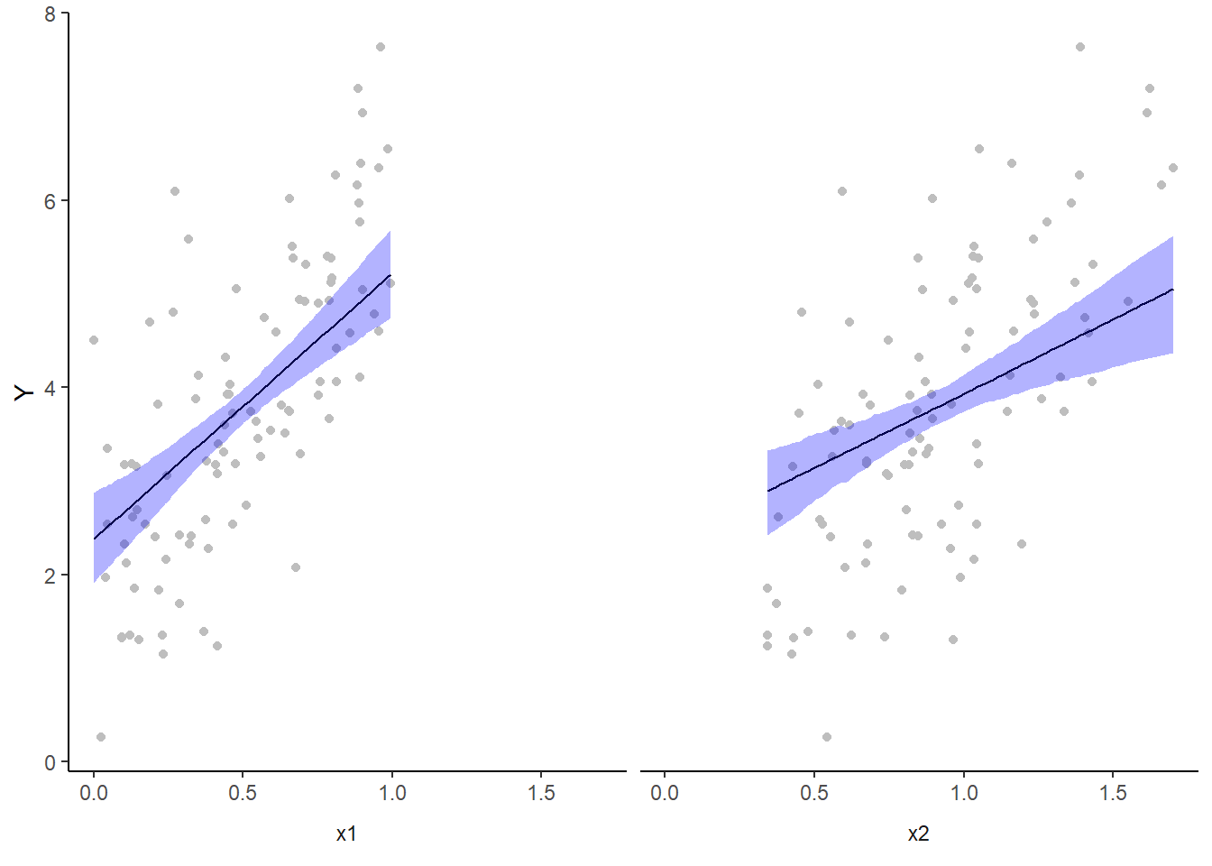
However, this method (whist partially elegant) does become overly opaque if we need more extensive axes labels since the x-axes labels are actually strip labels (which must largely be defined outside of the ggplot structure). The alternative is to simply produce each partial plot separately before arranging them together in the one figure using the package gridExtra.
> library(gridExtra)
> mcmc = as.matrix(data.rstan.add)
> ## Calculate the fitted values
> newdata = data.frame(cx1 = seq(min(data$cx1, na.rm = TRUE), max(data$cx1,
+     na.rm = TRUE), len = 100), cx2 = 0)
> Xmat = model.matrix(~cx1 + cx2, newdata)
> coefs = mcmc[, c("beta0", "beta[1]", "beta[2]")]
> fit = coefs %*% t(Xmat)
> newdata = newdata %>% mutate(x1 = cx1 + mean.x1, x2 = cx2 + mean.x2) %>%
+     cbind(tidyMCMC(fit, conf.int = TRUE, conf.method = "HPDinterval"))
> ## Now the partial residuals
> fdata = rdata = data.frame(cx1 = data$cx1, cx2 = 0)
> fMat = rMat = model.matrix(~cx1 + cx2, fdata)
> fit = as.vector(apply(coefs, 2, median) %*% t(fMat))
> resid = as.vector(data$y - apply(coefs, 2, median) %*% t(rMat))
> rdata = rdata %>% mutate(partial.resid = resid + fit) %>% mutate(x1 = cx1 +
+     mean.x1, x2 = cx2 + mean.x2)
> g1 = ggplot(newdata, aes(y = estimate, x = x1)) + geom_point(data = rdata,
+     aes(y = partial.resid), color = "grey") + geom_line() + geom_ribbon(aes(ymin = conf.low,
+     ymax = conf.high), fill = "blue", alpha = 0.3) + scale_y_continuous("Y") +
+     scale_x_continuous("X1") + theme_classic()
>
> newdata = data.frame(cx2 = seq(min(data$cx2, na.rm = TRUE), max(data$cx2,
+     na.rm = TRUE), len = 100), cx1 = 0)
> Xmat = model.matrix(~cx1 + cx2, newdata)
> coefs = mcmc[, c("beta0", "beta[1]", "beta[2]")]
> fit = coefs %*% t(Xmat)
> newdata = newdata %>% mutate(x1 = cx1 + mean.x1, x2 = cx2 + mean.x2) %>%
+     cbind(tidyMCMC(fit, conf.int = TRUE, conf.method = "HPDinterval"))
> ## Now the partial residuals
> fdata = rdata = data.frame(cx1 = 0, cx2 = data$cx2)
> fMat = rMat = model.matrix(~cx1 + cx2, fdata)
> fit = as.vector(apply(coefs, 2, median) %*% t(fMat))
> resid = as.vector(data$y - apply(coefs, 2, median) %*% t(rMat))
> rdata = rdata %>% mutate(partial.resid = resid + fit) %>% mutate(x1 = cx1 +
+     mean.x1, x2 = cx2 + mean.x2)
> g2 = ggplot(newdata, aes(y = estimate, x = x2)) + geom_point(data = rdata,
+     aes(y = partial.resid), color = "grey") + geom_line() + geom_ribbon(aes(ymin = conf.low,
+     ymax = conf.high), fill = "blue", alpha = 0.3) + scale_y_continuous("Y") +
+     scale_x_continuous("X2") + theme_classic()
>
> grid.arrange(g1, g2, ncol = 2)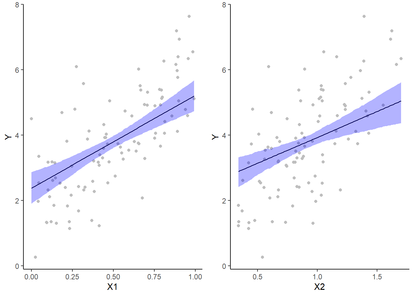
For the multiplicative model, we could elect to split the trends up so as to explore the effects of one predictor at several set levels of another predictor. In this example, we will explore the effects of \(x_1\) when \(x_2\) is equal to its mean in the original data as well as one and two standard deviations below and above this mean.
> library(fields)
> mcmc = as.matrix(data.rstan.mult)
> ## Calculate the fitted values
> newdata = expand.grid(cx1 = seq(min(data$cx1, na.rm = TRUE), max(data$cx1,
+     na.rm = TRUE), len = 100), cx2 = mean(data$cx2) + sd(data$cx2) %*%
+     -2:2)
> Xmat = model.matrix(~cx1 * cx2, newdata)
> coefs = mcmc[, c("beta0", "beta[1]", "beta[2]", "beta[3]")]
> fit = coefs %*% t(Xmat)
> newdata = newdata %>% mutate(x1 = cx1 + mean.x1, x2 = cx2 + mean.x2) %>%
+     cbind(tidyMCMC(fit, conf.int = TRUE, conf.method = "HPDinterval")) %>%
+     mutate(x2 = factor(x2, labels = paste("X2:~", c(-2, -1, 0, 1, 2), "*sigma")))
> ## Partial residuals
> fdata = rdata = expand.grid(cx1 = data$cx1, cx2 = mean(data$cx2) + sd(data$cx2) *
+     -2:2)
> fMat = rMat = model.matrix(~cx1 * cx2, fdata)
> fit = as.vector(apply(coefs, 2, median) %*% t(fMat))
> resid = as.vector(data$y - apply(coefs, 2, median) %*% t(rMat))
> rdata = rdata %>% mutate(partial.resid = resid + fit) %>% mutate(x1 = cx1 +
+     mean.x1, x2 = cx2 + mean.x2)
> ## Partition the partial residuals such that each x1 trend only includes
> ## x2 data that is within that range in the observed data
> findNearest = function(x, y) {
+     ff = fields:::rdist(x, y)
+     apply(ff, 1, function(x) which(x == min(x)))
+ }
> fn = findNearest(x = data[, c("x1", "x2")], y = rdata[, c("x1", "x2")])
> rdata = rdata[fn, ] %>% mutate(x2 = factor(x2, labels = paste("X2:~", c(-2,
+     -1, 0, 1, 2), "*sigma")))
> ggplot(newdata, aes(y = estimate, x = x1)) + geom_line() + geom_blank(aes(y = 9)) +
+     geom_point(data = rdata, aes(y = partial.resid), color = "grey") +
+     geom_ribbon(aes(ymin = conf.low, ymax = conf.high), fill = "blue",
+         alpha = 0.3) + scale_y_continuous("Y") + scale_x_continuous("X1") +
+     facet_wrap(~x2, labeller = label_parsed, nrow = 1, scales = "free_y") +
+     theme_classic() + theme(strip.background = element_blank())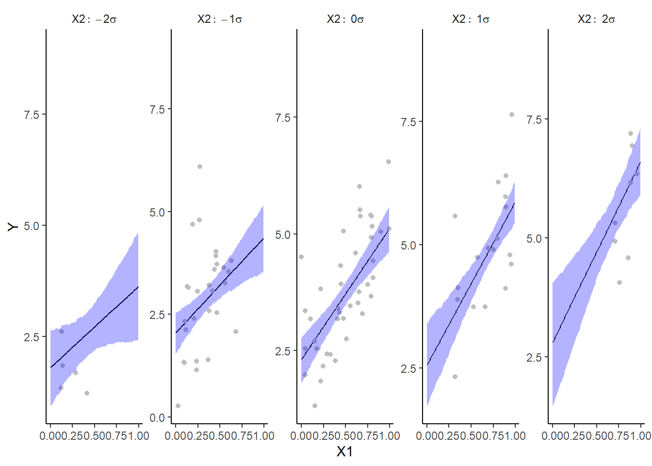
Alternatively, we could explore the interaction by plotting a two dimensional surface as a heat map.
Effect sizes
In addition to deriving the distribution means for the slope parameter, we could make use of the Bayesian framework to derive the distribution of the effect size. In so doing, effect size could be considered as either the rate of change or alternatively, the difference between pairs of values along the predictor gradient. For the latter case, there are multiple ways of calculating an effect size, but the two most common are:
Raw effect size. The difference between two groups (as already calculated)
Cohen’s D. The effect size standardized by division with the pooled standard deviation: \(D=\frac{(\mu_A-\mu_B)}{\sigma}\)
Percentage change. Express the effect size as a percent of one of the pairs. That is, whether you expressing a percentage increase or a percentage decline depends on which of the pairs of values are considered a reference value. Care must be exercised to ensure no division by zeros occur.
For simple linear models, effect size based on a rate is essentially the same as above except that it is expressed per unit of the predictor. Of course in many instances, one unit change in the predictor represents too subtle a shift in the underlying gradient to likely yield any clinically meaningful or appreciable change in response.
Probability that a change in \(x_1\) is associated with greater than a \(50\)% increase in \(y\) at various levels of \(x_2\). Clearly, in order to explore this inference, we must first express the change in \(y\) as a percentage. This in turn requires us to calculate start and end points from which to calculate the magnitude of the effect (amount of increase in \(y\)) as well as the percentage decline. Hence, we start by predicting the distribution of \(y\) at the lowest and highest values of \(x_1\) at five levels of \(x_2\) (representing two standard deviations below the cx2 mean, one standard deviation below the cx2 mean, the cx2 mean, one standard deviation above the cx2 mean and \(2\) standard deviations above the cx2 mean. For this exercise we will only use the multiplicative model. Needless to say, the process would be very similar for the additive model.
> mcmc = as.matrix(data.rstan.mult)
> newdata = expand.grid(cx1 = c(min(data$cx1), max(data$cx1)), cx2 = (-2:2) *
+     sd(data$cx1))
> Xmat = model.matrix(~cx1 * cx2, newdata)
> coefs = mcmc[, c("beta0", "beta[1]", "beta[2]", "beta[3]")]
> fit = coefs %*% t(Xmat)
> s1 = seq(1, 9, b = 2)
> s2 = seq(2, 10, b = 2)
> ## Raw effect size
> (RES = tidyMCMC(as.mcmc(fit[, s2] - fit[, s1]), conf.int = TRUE, conf.method = "HPDinterval"))
# A tibble: 5 x 5
  term  estimate std.error conf.low conf.high
  <chr>    <dbl>     <dbl>    <dbl>     <dbl>
1 2         1.95     0.825    0.301      3.52
2 4         2.37     0.568    1.25       3.50
3 6         2.80     0.441    1.91       3.59
4 8         3.22     0.546    2.18       4.32
5 10        3.64     0.796    2.16       5.28
> ## Cohen's D
> cohenD = (fit[, s2] - fit[, s1])/sqrt(mcmc[, "sigma"])
> (cohenDES = tidyMCMC(as.mcmc(cohenD), conf.int = TRUE, conf.method = "HPDinterval"))
# A tibble: 5 x 5
  term  estimate std.error conf.low conf.high
  <chr>    <dbl>     <dbl>    <dbl>     <dbl>
1 2         1.96     0.831    0.331      3.57
2 4         2.39     0.578    1.35       3.62
3 6         2.82     0.457    2.01       3.77
4 8         3.25     0.563    2.20       4.39
5 10        3.67     0.810    2.01       5.21
> # Percentage change (relative to Group A)
> ESp = 100 * (fit[, s2] - fit[, s1])/fit[, s1]
> (PES = tidyMCMC(as.mcmc(ESp), conf.int = TRUE, conf.method = "HPDinterval"))
# A tibble: 5 x 5
  term  estimate std.error conf.low conf.high
  <chr>    <dbl>     <dbl>    <dbl>     <dbl>
1 2         104.      74.7    -1.98      258.
2 4         113.      40.6    44.5       201.
3 6         121.      32.9    64.8       186.
4 8         128.      46.4    58.5       228.
5 10        133.      79.8    37.7       283.
> # Probability that the effect is greater than 50% (an increase of >50%)
> (p50 = apply(ESp, 2, function(x) sum(x > 50)/length(x)))
        2         4         6         8        10
0.8470000 0.9753333 0.9976667 0.9963333 0.9796667
> ## fractional change
> (FES = tidyMCMC(as.mcmc(fit[, s2]/fit[, s1]), conf.int = TRUE, conf.method = "HPDinterval"))
# A tibble: 5 x 5
  term  estimate std.error conf.low conf.high
  <chr>    <dbl>     <dbl>    <dbl>     <dbl>
1 2         2.04     0.747    0.980      3.58
2 4         2.13     0.406    1.45       3.01
3 6         2.21     0.329    1.65       2.86
4 8         2.28     0.464    1.58       3.28
5 10        2.33     0.798    1.38       3.83
Conclusions
On average, when \(x_2\) is equal to its mean, \(Y\) increases by \(2.79\) over the observed range of \(x_1\). We are \(95\)% confident that the increase is between \(1.91\) and \(3.66\).
The Cohen’s D associated change over the observed range of \(x_1\) is \(2.80\).
On average, \(Y\) increases by \(124\)% over the observed range of \(x_1\) (at average \(x_2\)). We are \(95\)% confident that the increase is between \(65\)% and \(190\)%.
The probability that \(Y\) increases by more than \(50\)% over the observed range of \(x_1\) (average \(x_2\)) is \(0.998\).
On average, \(Y\) increases by a factor of \(2.24\)% over the observed range of \(x_1\) (average \(x_2\)). We are \(95\)% confident that the decline is between a factor of \(1.65\)% and \(2.90\)%.
Finite population standard deviations
Variance components, the amount of added variance attributed to each influence, are traditionally estimated for so called random effects. These are the effects for which the levels employed in the design are randomly selected to represent a broader range of possible levels. For such effects, effect sizes (differences between each level and a reference level) are of little value. Instead, the “importance” of the variables are measured in units of variance components. On the other hand, regular variance components for fixed factors (those whose measured levels represent the only levels of interest) are not logical - since variance components estimate variance as if the levels are randomly selected from a larger population. Nevertheless, in order to compare and contrast the scale of variability of both fixed and random factors, it is necessary to measure both on the same scale (sample or population based variance).
Finite-population variance components assume that the levels of all factors (fixed and random) in the design are all the possible levels available (Gelman and others (2005)). In other words, they are assumed to represent finite populations of levels. Sample (rather than population) statistics are then used to calculate these finite-population variances (or standard deviations). Since standard deviation (and variance) are bound at zero, standard deviation posteriors are typically non-normal. Consequently, medians and HPD intervals are more robust estimates.
# A tibble: 4 x 5
  term     estimate std.error  conf.low conf.high
  <chr>       <dbl>     <dbl>     <dbl>     <dbl>
1 sd.x1       0.804    0.127  0.549         1.03
2 sd.x2       0.493    0.128  0.255         0.753
3 sd.x1x2     0.130    0.0881 0.0000621     0.294
4 sd.resid    0.977    0.0123 0.966         1.00
# A tibble: 4 x 5
  term     estimate std.error conf.low conf.high
  <chr>       <dbl>     <dbl>    <dbl>     <dbl>
1 sd.x1       33.3       4.91 23.2          42.4
2 sd.x2       20.5       5.11 11.4          31.2
3 sd.x1x2      5.37      3.46  0.00253      11.7
4 sd.resid    40.5       2.10 36.6          44.5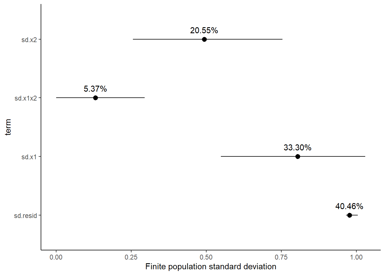
Approximately \(59\)% of the total finite population standard deviation is due to \(x_1\), \(x_2\) and their interaction.
R squared
In a frequentist context, the \(R^2\) value is seen as a useful indicator of goodness of fit. Whilst it has long been acknowledged that this measure is not appropriate for comparing models (for such purposes information criterion such as AIC are more appropriate), it is nevertheless useful for estimating the amount (percent) of variance explained by the model. In a frequentist context, \(R^2\) is calculated as the variance in predicted values divided by the variance in the observed (response) values. Unfortunately, this classical formulation does not translate simply into a Bayesian context since the equivalently calculated numerator can be larger than the an equivalently calculated denominator - thereby resulting in an \(R^2\) greater than \(100\)%. Gelman et al. (2019) proposed an alternative formulation in which the denominator comprises the sum of the explained variance and the variance of the residuals.
So in the standard regression model notation of:
\[ y_i \sim \text{Normal}(\boldsymbol X \boldsymbol \beta, \sigma),\]
the \(R^2\) could be formulated as
\[ R^2 = \frac{\sigma^2_f}{\sigma^2_f + \sigma^2_e},\]
where \(\sigma^2_f=\text{var}(\boldsymbol X \boldsymbol \beta)\), and for normal models \(\sigma^2_e=\text{var}(y-\boldsymbol X \boldsymbol \beta)\)
> mcmc <- as.matrix(data.rstan.mult)
> Xmat = model.matrix(~cx1 * cx2, data)
> coefs = mcmc[, c("beta0", "beta[1]", "beta[2]", "beta[3]")]
> fit = coefs %*% t(Xmat)
> resid = sweep(fit, 2, data$y, "-")
> var_f = apply(fit, 1, var)
> var_e = apply(resid, 1, var)
> R2 = var_f/(var_f + var_e)
> tidyMCMC(as.mcmc(R2), conf.int = TRUE, conf.method = "HPDinterval")
# A tibble: 1 x 5
  term  estimate std.error conf.low conf.high
  <chr>    <dbl>     <dbl>    <dbl>     <dbl>
1 var1     0.610    0.0381    0.532     0.676
>
> # for comparison with frequentist
> summary(lm(y ~ cx1 * cx2, data))

Call:
lm(formula = y ~ cx1 * cx2, data = data)

Residuals:
    Min      1Q  Median      3Q     Max
-1.8173 -0.7167 -0.1092  0.5890  3.3861

Coefficients:
            Estimate Std. Error t value Pr(>|t|)
(Intercept)   3.7152     0.1199  30.987  < 2e-16 ***
cx1           2.8072     0.4390   6.394 5.84e-09 ***
cx2           1.4988     0.3810   3.934 0.000158 ***
cx1:cx2       1.4464     1.1934   1.212 0.228476
---
Signif. codes:  0 '***' 0.001 '**' 0.01 '*' 0.05 '.' 0.1 ' ' 1

Residual standard error: 0.9804 on 96 degrees of freedom
Multiple R-squared:  0.6115,    Adjusted R-squared:  0.5994
F-statistic: 50.37 on 3 and 96 DF,  p-value: < 2.2e-16
Bayesian model selection
A statistical model is by definition a low-dimensional (over simplification) representation of what is really likely to be a very complex system. As a result, no model is right. Some models however can provide useful insights into some of the processes operating on the system. Frequentist statistics have various methods (model selection, dredging, lasso, cross validation) for selecting parsimonious models. These are models that provide a good comprimise between minimizing unexplained patterns and minimizing model complexity. The basic premise is that since no model can hope to capture the full complexity of a system with all its subtleties, only the very major patterns can be estimated. Overly complex models are likely to be representing artificial complexity present only in the specific observed data (not the general population). The Bayesian approach is to apply priors to the non-variance parameters such that parameters close to zero are further shrunk towards zero whilst priors on parameters further away from zero are less effected. The most popular form of prior for sparsity is the horseshoe prior, so called because the shape of a component of this prior resembles a horseshoe (with most of the mass either close to \(0\) or close to \(1\)).
Rather than apply weakly informative Gaussian priors on parameters as:
\[ \beta_j \sim N(0,\sigma^2),\]
the horseshoe prior is defined as
\[ \beta_j \sim N(0,\tau^2\lambda_j^2),\]
where \(\tau \sim \text{Cauchy}(0,1)\) and \(\lambda_j \sim \text{Cauchy}(0,1)\), for \(j=1,\ldots,D\). Using this prior, \(D\) is the number of (non-intercept or variance) parameters, \(\tau\) represents the global scale that weights or shrinks all parameters towards zero and \(\lambda_j\) are thick tailed local scales that allow some of the \(j\) parameters to escape shrinkage. More recently, Piironen, Vehtari, and others (2017) have argued that whilst the above horseshoe priors do guarantee that strong effects (parameters) will not be over-shrunk, there is the potential for weekly identified effects (those based on relatively little data) to be misrepresented in the posteriors. As an alternative they advocated the use of regularised horseshoe priors in which the amount of shrinkage applied to the largest effects can be controlled. The prior is defined as:
\[ \beta_j \sim N(0,\tau^2 \tilde{\lambda}_j^2),\]
where \(\tilde{\lambda}_j^2 = \frac{c^2\lambda^2_j}{c^2+\tau^2 \lambda^2_j}\) and \(c\) is (slab width, actually variance) is a constant. For small effects (when \(\tau^2 \lambda^2_j < c^2\)) the prior approaches a regular prior. However, for large effects (when \(\tau^2 \lambda^2_j > c^2\)) the prior approaches \(N(0,c^2)\). Finally, they recommend applying a inverse-gamma prior on \(c^2\):
\[ c^2 \sim \text{Inv-Gamma}(\alpha,\beta),\]
where \(\alpha=v/2\) and \(\beta=vs^2/2\), which translates to a \(\text{Student-t}_ν(0, s^2)\) slab for the coefficients far from zero and is typically a good default choice for a weakly informative prior. This prior can be encoded into Stan using the following code.
> modelStringHP = "
+                        data {
+                        int < lower =0 > n; // number of observations
+                        int < lower =0 > nX; // number of predictors
+                        vector [ n] Y; // outputs
+                        matrix [n ,nX] X; // inputs
+                        real < lower =0 > scale_icept ; // prior std for the intercept
+                        real < lower =0 > scale_global ; // scale for the half -t prior for tau
+                        real < lower =1 > nu_global ; // degrees of freedom for the half -t priors for tau
+                        real < lower =1 > nu_local ; // degrees of freedom for the half - t priors for lambdas
+                        real < lower =0 > slab_scale ; // slab scale for the regularized horseshoe
+                        real < lower =0 > slab_df ; // slab degrees of freedom for the regularized horseshoe
+                        }
+                        transformed data {
+                        matrix[n, nX - 1] Xc;  // centered version of X
+                        vector[nX - 1] means_X;  // column means of X before centering
+                        for (i in 2:nX) {
+                        means_X[i - 1] = mean(X[, i]);
+                        Xc[, i - 1] = X[, i] - means_X[i - 1];
+                        }
+                        }
+                        parameters {
+                        real logsigma ;
+                        real cbeta0 ;
+                        vector [ nX-1] z;
+                        real < lower =0 > tau ; // global shrinkage parameter
+                        vector < lower =0 >[ nX-1] lambda ; // local shrinkage parameter
+                        real < lower =0 > caux ;
+                        }
+                        transformed parameters {
+                        real < lower =0 > sigma ; // noise std
+                        vector < lower =0 >[ nX-1] lambda_tilde ; // truncated local shrinkage parameter
+                        real < lower =0 > c; // slab scale
+                        vector [ nX-1] beta ; // regression coefficients
+                        vector [ n] mu; // latent function values
+                        sigma = exp ( logsigma );
+                        c = slab_scale * sqrt ( caux );
+                        lambda_tilde = sqrt ( c ^2 * square ( lambda ) ./ (c ^2 + tau ^2* square ( lambda )) );
+                        beta = z .* lambda_tilde * tau ;
+                        mu = cbeta0 + Xc* beta ;
+                        }
+                        model {
+                        // half -t priors for lambdas and tau , and inverse - gamma for c ^2
+                        z ~ normal (0 , 1);
+                        lambda ~ student_t ( nu_local , 0, 1);
+                        tau ~ student_t ( nu_global , 0 , scale_global * sigma );
+                        caux ~ inv_gamma (0.5* slab_df , 0.5* slab_df );
+                        cbeta0 ~ normal (0 , scale_icept );
+                        Y ~ normal (mu , sigma );
+                        }
+                        generated quantities {
+                        real beta0;  // population-level intercept
+                        vector[n] log_lik;
+                        beta0 = cbeta0 - dot_product(means_X, beta);
+                        for (i in 1:n) {
+                        log_lik[i] = normal_lpdf(Y[i] | Xc[i] * beta + cbeta0, sigma);
+                        }
+                        }
+
+   "
> ## write the model to a stan file
> writeLines(modelStringHP, con = "linregModelHP.stan")
We can now try to refit the model (additive) using this new specification.
> X = model.matrix(~cx1 + cx2, data = data)
> data.list <- with(data, list(Y = y, X = X, nX = ncol(X), n = nrow(data),
+     scale_icept = 100, scale_global = 1, nu_global = 1, nu_local = 1, slab_scale = 2,
+     slab_df = 4))
>
> data.rstan.sparsity <- stan(data = data.list, file = "linregModelHP.stan", pars = params,
+     chains = nChains, iter = nIter, warmup = burnInSteps, thin = thinSteps, save_dso = TRUE)

SAMPLING FOR MODEL 'linregModelHP' NOW (CHAIN 1).
Chain 1:
Chain 1: Gradient evaluation took 0.001 seconds
Chain 1: 1000 transitions using 10 leapfrog steps per transition would take 10 seconds.
Chain 1: Adjust your expectations accordingly!
Chain 1:
Chain 1:
Chain 1: Iteration:    1 / 2500 [  0%]  (Warmup)
Chain 1: Iteration:  250 / 2500 [ 10%]  (Warmup)
Chain 1: Iteration:  500 / 2500 [ 20%]  (Warmup)
Chain 1: Iteration:  750 / 2500 [ 30%]  (Warmup)
Chain 1: Iteration: 1000 / 2500 [ 40%]  (Warmup)
Chain 1: Iteration: 1001 / 2500 [ 40%]  (Sampling)
Chain 1: Iteration: 1250 / 2500 [ 50%]  (Sampling)
Chain 1: Iteration: 1500 / 2500 [ 60%]  (Sampling)
Chain 1: Iteration: 1750 / 2500 [ 70%]  (Sampling)
Chain 1: Iteration: 2000 / 2500 [ 80%]  (Sampling)
Chain 1: Iteration: 2250 / 2500 [ 90%]  (Sampling)
Chain 1: Iteration: 2500 / 2500 [100%]  (Sampling)
Chain 1:
Chain 1:  Elapsed Time: 0.296 seconds (Warm-up)
Chain 1:                0.374 seconds (Sampling)
Chain 1:                0.67 seconds (Total)
Chain 1:

SAMPLING FOR MODEL 'linregModelHP' NOW (CHAIN 2).
Chain 2:
Chain 2: Gradient evaluation took 0 seconds
Chain 2: 1000 transitions using 10 leapfrog steps per transition would take 0 seconds.
Chain 2: Adjust your expectations accordingly!
Chain 2:
Chain 2:
Chain 2: Iteration:    1 / 2500 [  0%]  (Warmup)
Chain 2: Iteration:  250 / 2500 [ 10%]  (Warmup)
Chain 2: Iteration:  500 / 2500 [ 20%]  (Warmup)
Chain 2: Iteration:  750 / 2500 [ 30%]  (Warmup)
Chain 2: Iteration: 1000 / 2500 [ 40%]  (Warmup)
Chain 2: Iteration: 1001 / 2500 [ 40%]  (Sampling)
Chain 2: Iteration: 1250 / 2500 [ 50%]  (Sampling)
Chain 2: Iteration: 1500 / 2500 [ 60%]  (Sampling)
Chain 2: Iteration: 1750 / 2500 [ 70%]  (Sampling)
Chain 2: Iteration: 2000 / 2500 [ 80%]  (Sampling)
Chain 2: Iteration: 2250 / 2500 [ 90%]  (Sampling)
Chain 2: Iteration: 2500 / 2500 [100%]  (Sampling)
Chain 2:
Chain 2:  Elapsed Time: 0.308 seconds (Warm-up)
Chain 2:                0.402 seconds (Sampling)
Chain 2:                0.71 seconds (Total)
Chain 2:
>
> tidyMCMC(data.rstan.sparsity, pars = c("beta[1]", "beta[2]"), conf.int = TRUE,
+     conf.type = "HPDinterval", rhat = TRUE, ess = TRUE)
# A tibble: 2 x 7
  term    estimate std.error conf.low conf.high  rhat   ess
  <chr>      <dbl>     <dbl>    <dbl>     <dbl> <dbl> <int>
1 beta[1]     2.76     0.439    1.90       3.61  1.00  3330
2 beta[2]     1.56     0.375    0.806      2.29  1.00  3086
>
> mcmc_areas(as.matrix(data.rstan.sparsity), regex_par = "beta")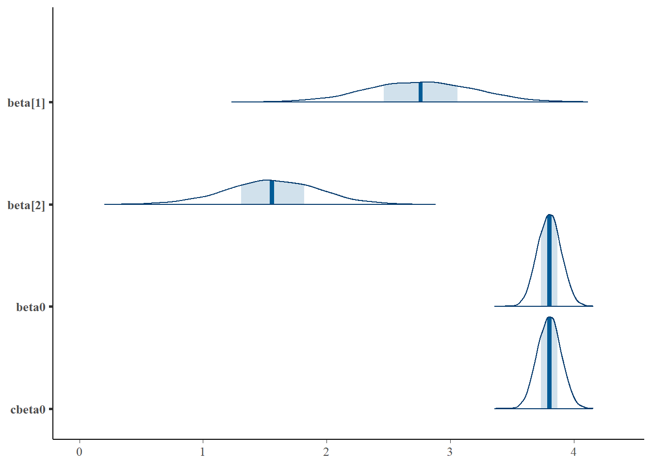
Obviously, these data are not really appropriate for model selection as there are only two predictors. Both predictors have substantial effects mass larger than zero.